NMRProcFlow Documentation
Warnings: be aware that this document has been automatically compiled from the online documentation as a single page, so there is no content table and some headers are missing.

About NMRProcFlow
© Copyright 2016-2021
Funded by:
- INRA UMR 1332 BFP, Bordeaux Metabolomics Facility
- the ANR-11-INBS-0010 grant (MetaboHUB)
Main contributors:
- Daniel Jacob
- Catherine Deborde
- Marie Lefebvre
- Michaël Maucourt
Special thanks to Alain Girard (INRA Bordeaux) for designing the logo.
Publication:
Jacob, D., Deborde, C., Lefebvre, M., Maucourt, M. and Moing, A. (2017) NMRProcFlow: A graphical and interactive tool dedicated to 1D spectra processing for NMR-based metabolomics, Metabolomics 13:36. doi:10.1007/s11306-017-1178-y
Call for contribution
We have been developing this software since 2015 and this requires a long and continuous effort. Firstly, our aim was to fulfill our own needs in the matter of NMR spectra processing, and we assume that it also meets your needs. Because no one can claim to have innate knowledge, we believe it is more beneficial for all to share our expertise. That's why we decided to give an open access of this software. So, this software is now a little yours too.
- An easy way to contribute is to keep trace of problems encountered with NMRProcFlow, and send them to us by email. Thus, it is a good way to ensure the development and the continual improvement of the NMRProcFlow system.
- Another way to contribute is to send us your suggestions about new functionalities that would be advisable to develop in priority, and those that must be improved.
- A third way to contribute is to propose your own R scripts or packages you would like to be integrated within the software in order to enrich the functionnalities.
- A last way to contribute is to become an NMRProcFlow developer (as soon as the code source will be opened).
Contact the maintainers: NMRProcFlow Team
Training
NMRProcFlow has been developed to meet some expert needs. Although a non-expert user can use it, basic skills in NMR spectra processing is nevertheless required to take full advantage of its possibilities. Given that NMRProcFlow will do what you ask it to do, no matter if this is coherent or absurd, we think it is unfortunately not a software that can fill such a lack, but indeed an appropriate training (Weber et al 2015).
It should be noted that the online version of NMRProcFlow is not dedicated to intensive use and therefore is not suitable for a workshop with more than 10 simultaneous sessions. Also, we highly recommend the local installation of the application. For those who would like to organize training sessions or workshops where NMRProcFlow would be used as a support tool, please, contact the NMRProcFlow Team to see which strategy would be best suited.
Weber, Ralf J. M., Winder, Catherine L., Larcombe, Lee D., Dunn, Warwick B., Viant, Mark R. (2015) Training needs in metabolomics, Metabolomics 11:784-786. doi:10.1007/s11306-015-0815-6
Futur work
We have planned to develop some functionalities in order to meet particular needs
- We already support the nmrML format nmrML for NMR spectra (FID). In a next version the final goal will to achieve a complete export in this new standard format, thus allowing to describe based on an ontology (nmrCV) the whole processing steps (ongoing work)
- Carry on the quantification (targeted metabolomics - qHNMR) based on signal deconvolution i.e. on line shape analysis of the signal (under study)
License:
- GNU GENERAL PUBLIC LICENSE Version 3, 29 June 2007 - See http://www.gnu.org/licenses/ for more details.

Overview
An user-friendly tool dedicated to 1D NMR spectra processing (1H, 13C, 31P)
for metabolomics
NMRProcFlow is an open source software that greatly helps spectra processing. It was built by involving NMR spectroscopists eager to have a quick and easy tool to use.
Given the nature of the 1D NMR spectra and due to the diversity of problems encountered during the various stages of processing:
- baseline correction,
- ppm calibration,
- removal of solvents and other contaminants
- re-alignment of areas having high variations in chemical shifts between spectra, ...
and depending on:
- the biological context (humans, plants, micro-organisms),
- the type of sample source (tissue or biofluid like plasma, urine, plant extracts ...),
- the analytical protocol (choice of NMR sequence, use of additives for calibration and / or quantification, use of buffer solution to stabilize pH, etc ...).
It is essential to process this type of data, with an interactive interface that enables spectra visualization.
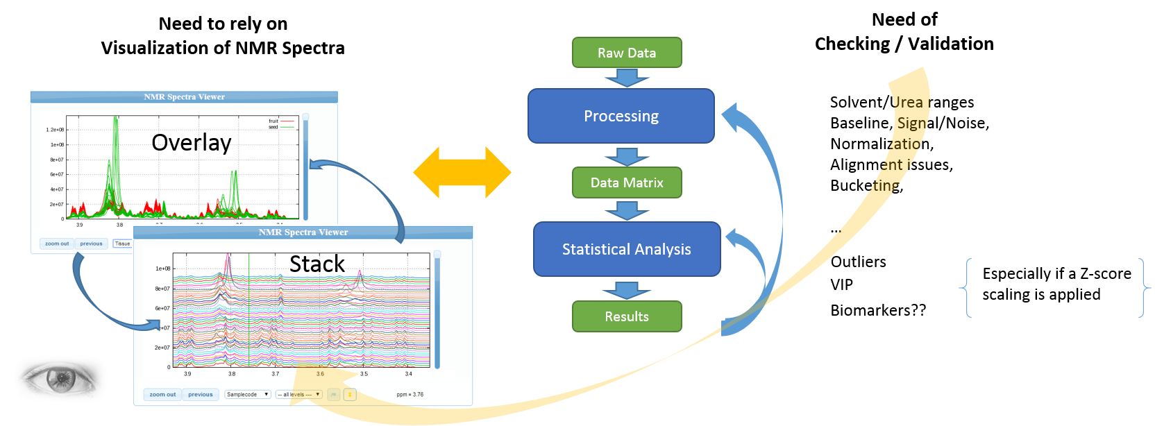
The expert's eyes are crucial to select the parameters, and to validate the treatments
Apart for very well-mastered and very reproducible use cases (see Batch mode execution), the implementation of NMR spectra processing workflows executed in batch mode (regarding as a black-box) seems to us very hazardous, and can produce output aberrations. So, it is crucial to proceed in an interactive way with a NMR spectra viewer to allow the expert eye to disentangle the intertwined peaks.
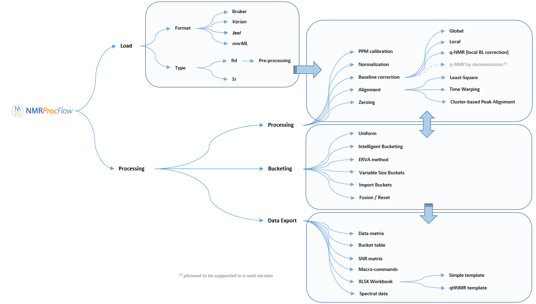
Major concerns having (initially) motivated the design and having served as a roadmap :
- Ease the data preparation phase in order to be loaded via the web interface
- View the spectra according to the experimental conditions, or separately,
- Allow user to apply interactive data processing procedures to all the spectra, either to the whole ppm range with the same set of parameters or to only a selected ppm range with specific set of parameters for each ppm range,
- Export a data matrix to establish statistical analysis ( (un)targeted approaches) with a statistical tool (such as BioStatFlow, MetaboAnalyst ...) so that the file manipulations are minimized.
- Allow user to replay the same processing workflow (e.g. few months later) on the same dataset or a similar one
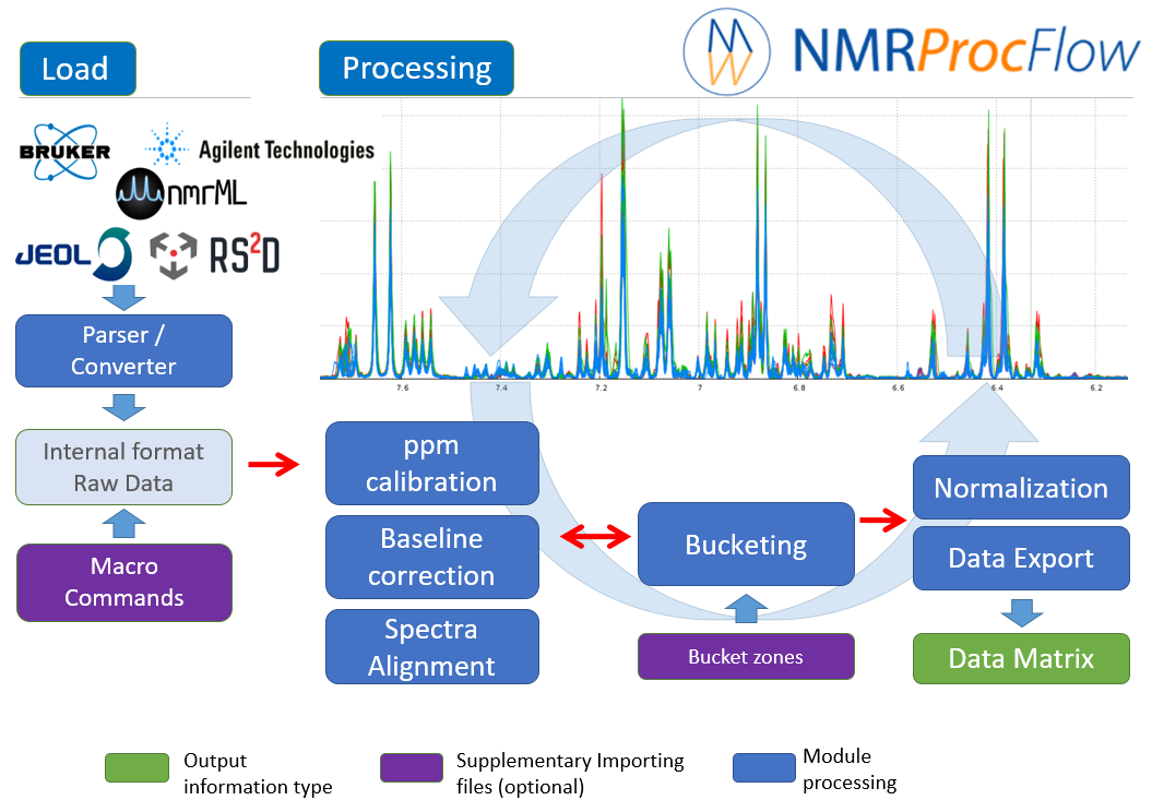
NMRProcFlow open source software provides a complete set of tools for processing and visualizing of 1D NMR data, within an interactive interface based on a spectra visualization.

Metabolomics approaches
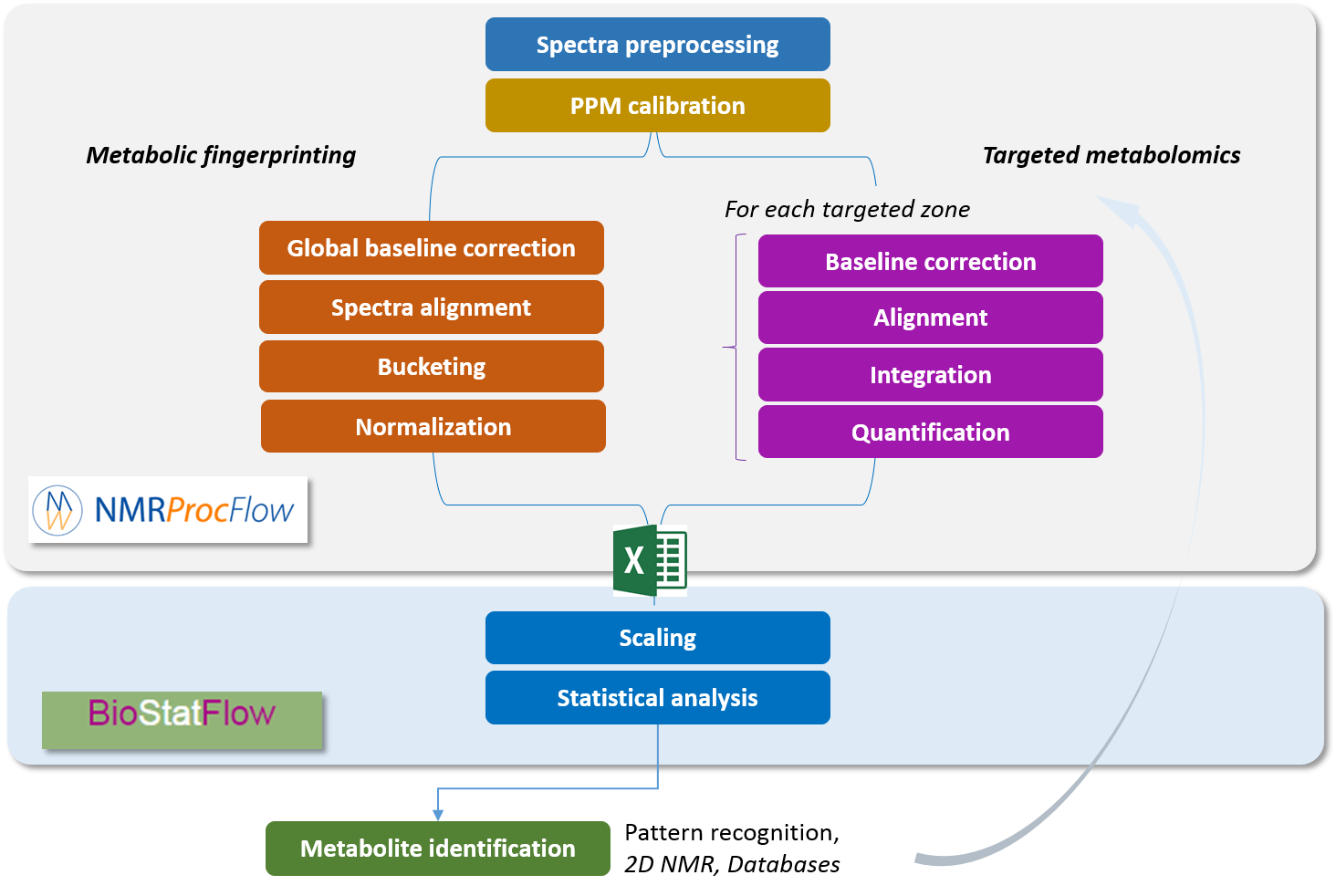
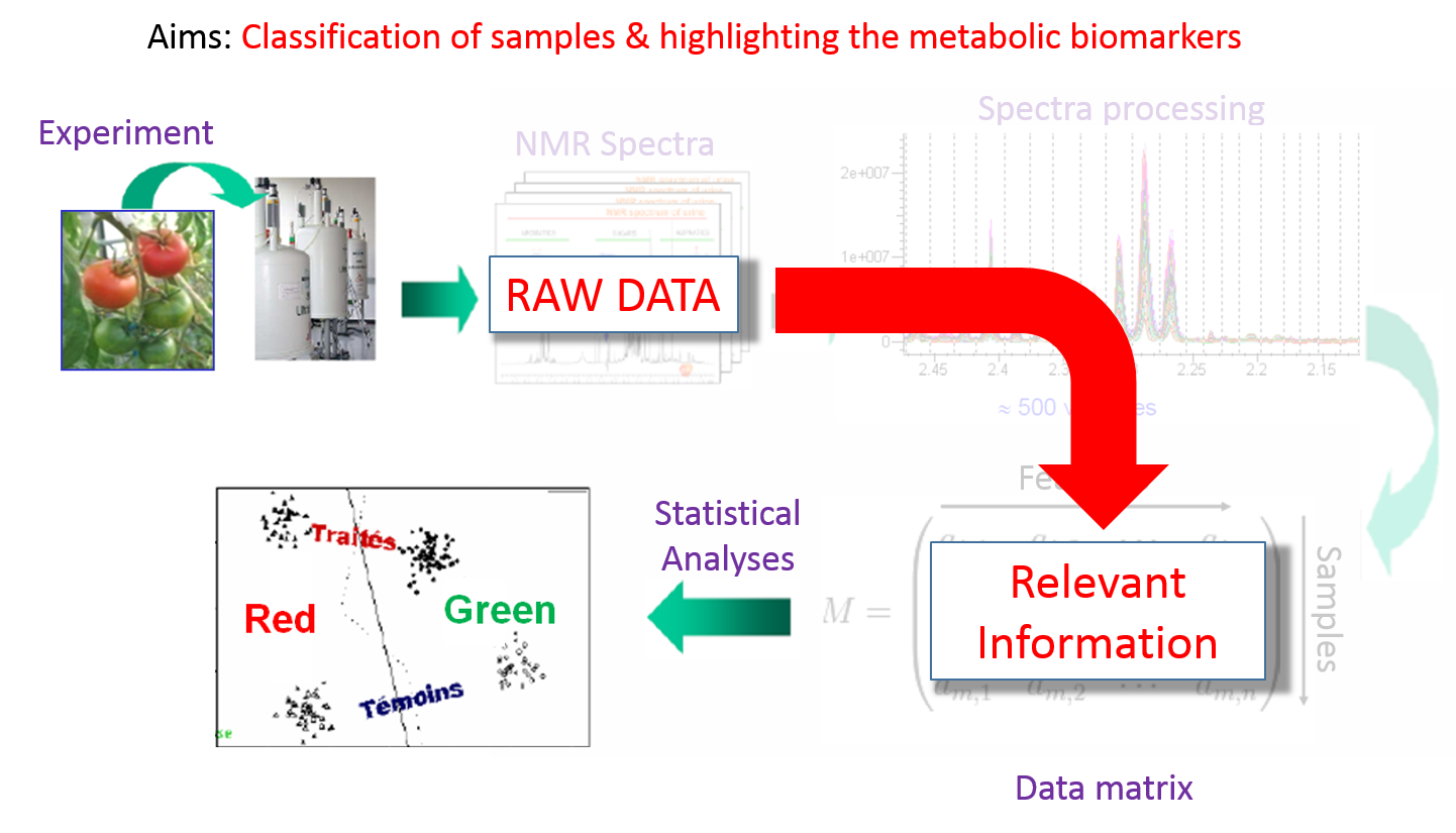
NMRProcFlow is especially dedicated to metabolomics. The two major metabolomics approaches, namely metabolic fingerprinting and targeted metabolomics are taken into account. The workflow covers all steps from the spectral data up to the output data matrix
|
Metabolic Fingerprinting The complex data are directly and initially used for global multivariate statistical analysis. Subsequently, metabolite features that distinguish sample classes are identified and then the structures of distinguishing metabolic features are established |
 |
Targeted Metabolomics Quantitative approach wherein a set of known metabolites are quantitated. The identities of metabolites were initially established based on the available databases and using standard compounds. The identified metabolite peaks are then quantified based on internal or external reference compounds. |
|
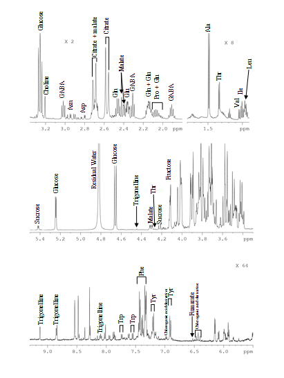 |
|
| See more ... | See more ... |

Metabolic Fingerprinting
Metabolic fingerprinting refers to the use of machine output as potentially recognizable chemical pattern, specific of an individual sample. Metabolite fingerprinting by NMR is a fast, convenient, and effective tool for discriminating between groups of related samples and it identifies the most important regions of the spectra for further analysis.
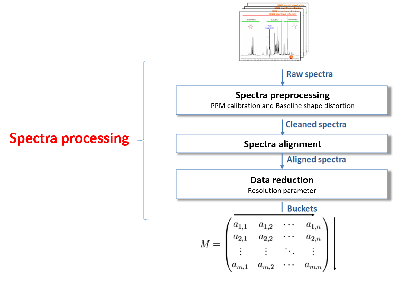
So the spectra processing is an intermediate step between raw spectra and data analysis. It consists to preserve as much as possible the variance relative to the chemical compounds contained in the NMR spectra while reducing other types of variance induced by different sources of bias such as baseline and misalignment. See Spectra processing section.
Then, the identity of the metabolites of interest is established after statistical data analysis of metabolic fingerprints, and this involves to be able:
- to highlight that spectral regions having a difference between the groups are statistically significant.
- to ensure that each of these regions involves only a single metabolite, i.e. there is unique correspondence between a bucket and a resonance (spectral signature) of a metabolite
The standard approach in NMR-based metabolomics implies the division of spectra into equally sized bins, thereby simplifying subsequent data analysis. Yet, disadvantages are the loss of information and the occurrence of artifacts caused by peak shifts. Therefore we implemented the Adaptive Intelligent Binning (AI-Binning) algorithm which largely circumvents these problems. It recursively identifies bin edges in existing bins, requires only minimal user input, and avoids the use of arbitrary parameters or reference spectra. This algorithm is well adapted to meet the second point mentioned above.
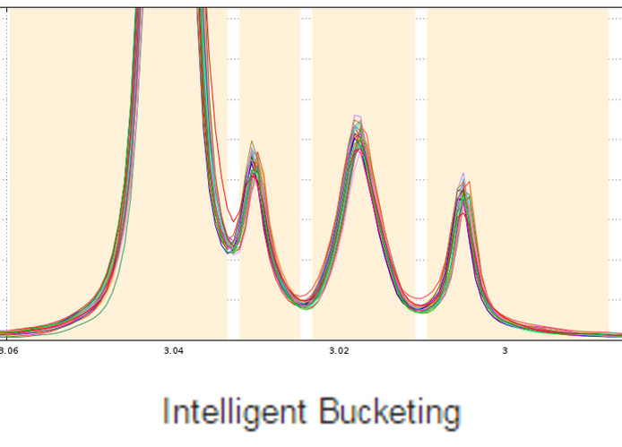
De Meyer T., Sinnaeve D., Gasse B., Tsiporkova E., Rietzschel E., De Buyzere M., Gillebert T., Bekaert S., Martins J. and Criekinge W. (2008) NMR-Based Characterization of Metabolic Alterations in Hypertension Using an Adaptive, Intelligent Binning Algorithm. Analytical Chemistry 80(10):3783–3790
How to further proceed ?
After the bucketing, you have to export the data matrix (see Export the Data matrix). The exported matrix is formatted so that we can subsequently perform statistical analysis using BioStatFlow (*) web application. Thus the data file manipulations are minimized.
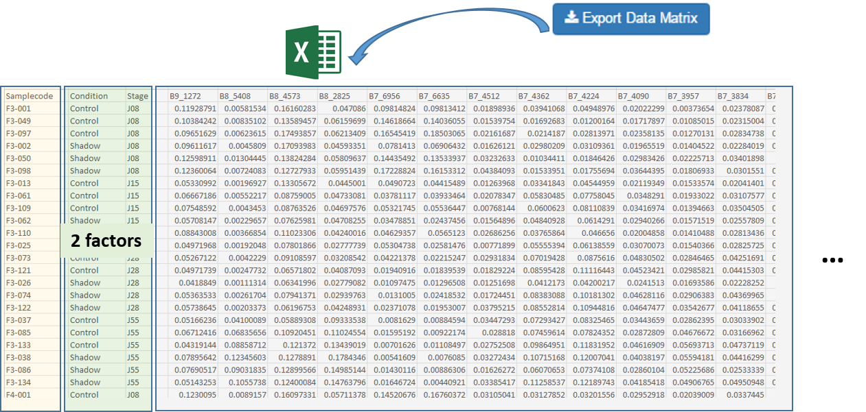
Import the Data Matrix to BioStatFlow
After exporting, the data matrix is formatted so that we can subsequently perform statistical analysis using BioStatFlow(*) web application. Thus the data file manipulations are minimized.
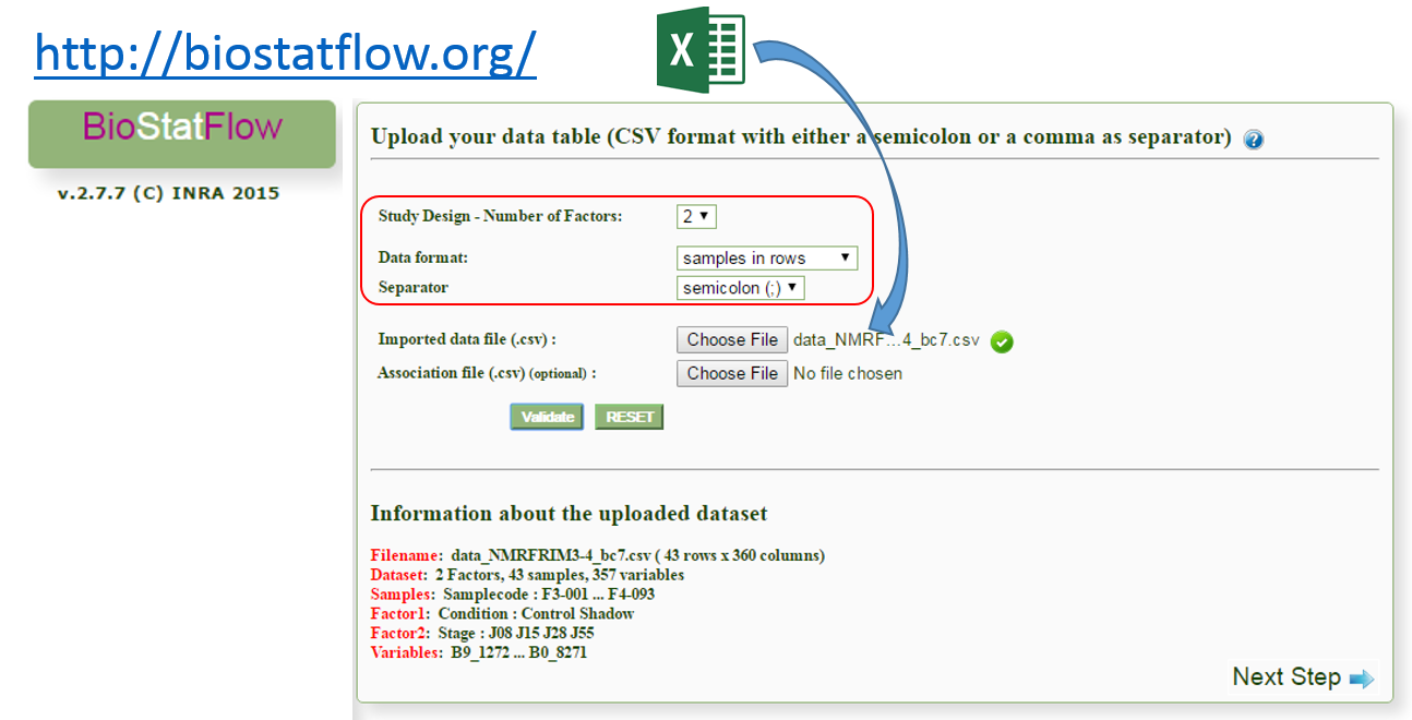
(*) See MetaboNews Issue 42 - February 2015
See online some slides showing a simple session of BioStatFlow in action: Example of a BioStatFlow session and the Help online of BioStatFlow
Import the Data Matrix to MetaboAnalyst
After exporting, the data matrix is formatted so that we can subsequently perform statistical analysis using MetaboAnalyst (Xia et al. 2015). See online some slides showing a simple session with MetaboAnalyst.
Xia, J., Sinelnikov, I., Han, B., and Wishart, D.S. (2015) MetaboAnalyst 3.0 - making metabolomics more meaningful . Nucl. Acids Res. 43, W251-257.
Help in the identification
Still in the embryonic stage, we currently develop tools that will greatly help in the identification. See online some slides showing about Help in the identification

Targeted Metabolomics
This refers to quantitative approaches wherein a set of known metabolites are quantitated. The identities of metabolites have been initially established based on the available databases and using standard compounds. The identified metabolite peaks are then quantified based on internal or external reference compounds. Here, we suggest two references as good reviews that could be read with great profit:
- Santosh Kumar Bharti, Raja Roy (2012) Quantitative 1H NMR, spectroscopy, Trends in Analytical Chemistry 35:5-26, doi:10.1016/j.trac.2012.02.007
- Patrick Giraudeau, Illa Tea, Gérald S. Remaud, Serge Akoka (2014) Reference and normalization methods: Essential tools
for the intercomparison of NMR spectra, Journal of Pharmaceutical and Biomedical Analysis 93:3–16, doi:10.1016/j.trac.2012.02.007
In this case the identity of the metabolites of interest is established before statistical data analysis, and this involves to be able:
- to identify the ppm areas for which the quantification will be performed based on both knowledge and well-established metabolomic profiles,
- to ensure that each of these areas is not polluted by the neighbor areas
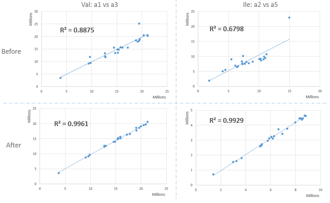
To fulfill these two points, it is necessary to locally correct the baseline in order to i) eliminate the residual effects due to the presence of macromolecules in extracts, ii) but also reduce the prevalence of a high intense peak on the less intense ones.
Example of local baseline correction for quantifying compounds via 1H NMR
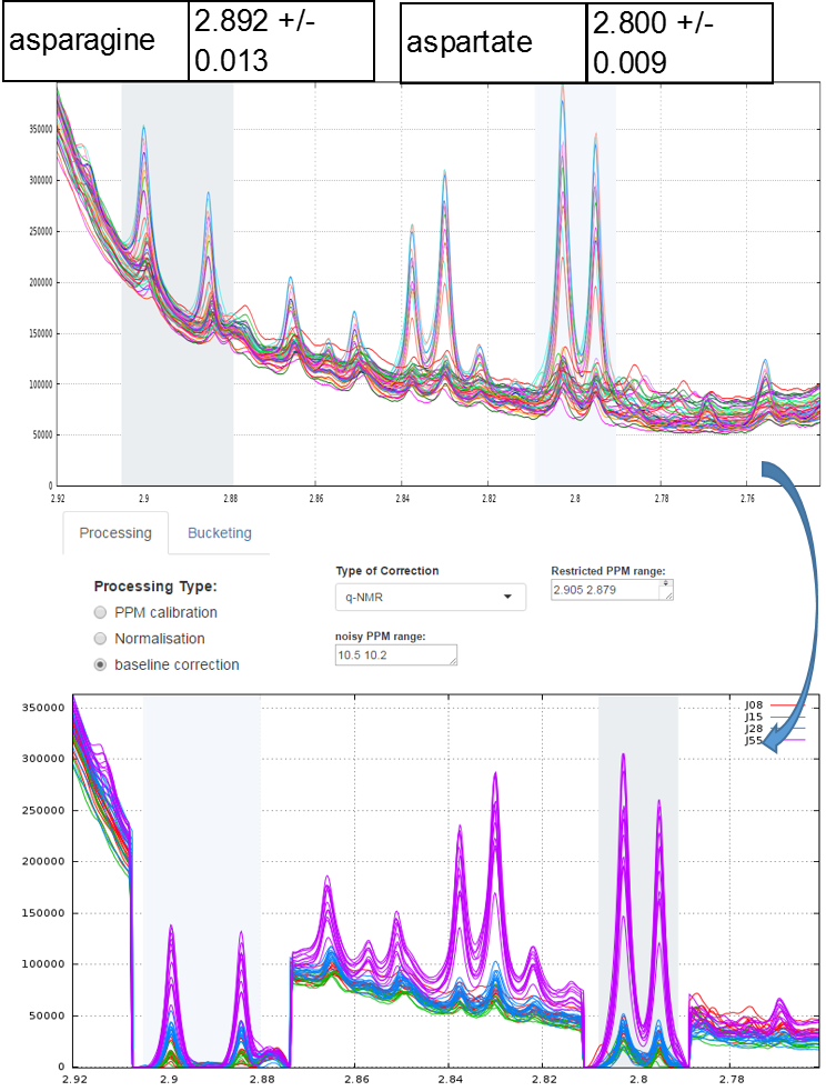
To quantify target compounds, a simple and efficient method is to fit the lineshape applied on a signal portion of those compounds. These signal portions are chosen such that they are not or little affected (ie in a smoothly way) by a possible overlap with a neighboring peak. In the figure below, the two targeted compounds (asparagine and aspartate) exhibit each of them a doublet whose only their lineshape are affects by the trailing signal of a high intensity nearby lorentizian.
Typical approach for quantifying compounds via 1H NMR
A typical approach for quantifying compounds via 1H NMR is based on Calibration-curve method (i.e. external reference optionaly coupled with an internal reference such as ERETIC). For more explanation and details, see the reference given above.
After the processing and bucketing steps, NMRProcFlow allows users to export all data needed for the quantification in a same XLSX workbook. Two workbook templates were currently available: A simple one and a template dedicated for the quantification.
- The simple template just aggregates the buckets table, the SNR matrix and the data matrix, each data type being within a separate tab.
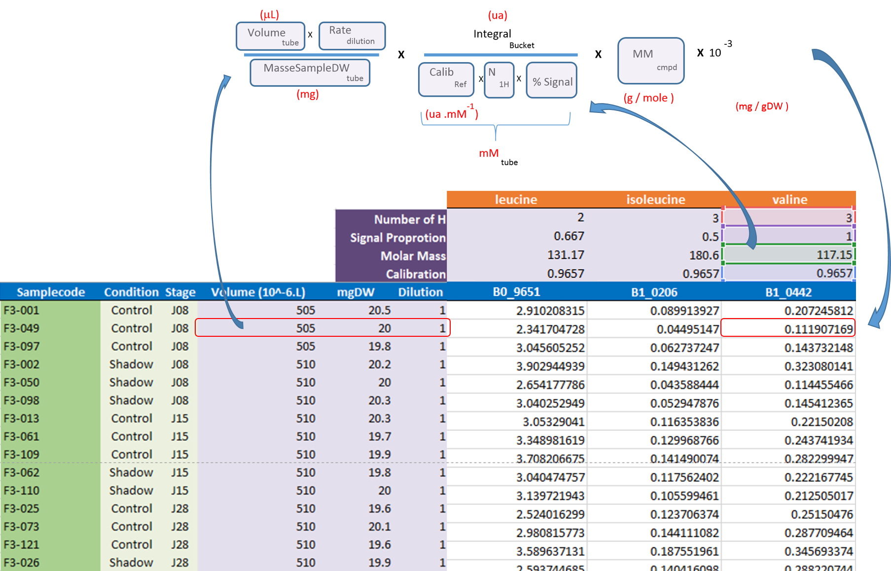
- The 'qHNMR' template, in the same way as the simple template aggregates information like the samples table, the buckets table, the SNR matrix and the data matrix within separate tabs, but also includes another tab with the pre-calculated quantications according to a formula from data provided in the others tabs. Some information are set by default in both 'samples' and 'buckets' tabs. Just adjust them with the appropriate values and the quantifications within the eponymous tab will be automatically updated as depicted in the figure below:
See online some slides about the targeted approach along with NMRProcFlow: Targeted metabolomics

Description of the implemented processing methods
NMRProcFlow provides a complete set of tools for processing 1D NMR data, the whole embedded within an interface allowing to interact with a spectra viewer.

Our criterion for the choice of methods for each spectra processing stage (baseline, alignment, binning ...) to implement in our application were those that:
- were evaluated as effective according to our tests,
- can be applied to both a small zone ( <0.5 ppm) or a large zone (several ppm),
- when applied on several dozen of spectra require only few seconds in their execution (implying an appropriate implementation) in order to allow a fluid use of the application.
When these methods were already implemented within a R package, then we integrated it. Otherwise, we implemented them ourselves in R / C ++.
Moreover, the expert's eyes are crucial to select the parameters, and to validate the treatments. Apart for very well-mastered and very reproducible use cases (see Batch mode execution), the implementation of NMR spectra processing workflows executed in batch mode (regarding as a black-box) seems to us very hazardous, and can produce output aberrations. So, it is crucial to proceed in an interactive way with a NMR spectra viewer to allow the expert eye to disentangle the intertwined peaks. Being the heart of our approach, this aspect of interactive visualization is central to our method choices.

1 - Spectra pre-processing
The spectral preprocessing for 1D NMR can be automatically applied in case the input raw data are FID, either from a Bruker or Varian spectrometer. The term pre-processing designates here the transformation of the NMR spectrum from time domain to frequency domain, including the phase correction and the fast Fourier-transform (FFT).
From the work of Hans de Brouwer et al (2009), the adapted then implemented algorithm follows the steps (i.e. from FID to the corresponding real spectrum) depicted by the figure below:
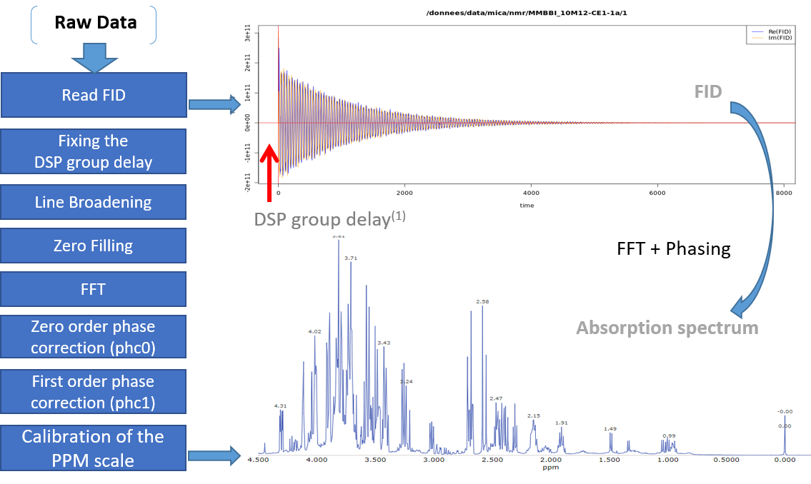
(1) In the case of Bruker spectra a death time or group delay can be observed in the FID.
Note: You can optimize the parameters to apply on your own raw spectra from the small application online at the URL https://pmb-bordeaux.fr/nmrspec/.
References
Hans de Brouwer et al (2009) Evaluation of algorithms for automated phase correction of NMR spectra doi:10.1016/j.jmr.2009.09.017, Journal of Magnetic Resonance 201(2):230-8

2 - Baseline correction
Two types of Baseline correction were implemented: Global and Local. To be more efficient, both methods need to estimate the noise level, and by default the spectral or ppm range considered, is between 10.2 and 10.5 ppm. But users can choose another spectral range if some signal is present in this area.
2.1 - Global baseline correction
The global baseline correction was based on [Bao et al., 2012], but only two phases were implemented: i) Continuous Wavelet Transform (CWT), and ii) the sliding window algorithm. The user must choose the correction level, from 'soft' up to 'high'.
2.2 - Local baseline correction
The airPLS (adaptive iteratively reweighted penalized least squares) algorithm based on [Zhang et al., 2010] is a baseline correction algorithm that works completely on its own, and that only requires a “detail” parameter for the algorithm, called Lambda. Because this Lambda parameter can vary within a very large range (from 10 up to 1.e+06), we converted this parameter within a more convenient scale for the user, called 'level correction factor' chosen by the user from '1' (soft) up to '6' (high). The lower this level correction factor is set, the smoother baseline will be. Conversely, the higher this level correction factor is set, the more baseline will be corrected in details. To be more efficient, the algorithm needs to estimate the noise level; by default the spectral or ppm range considered is between 10.2 and 10.5 ppm. However, users can choose another spectral range if some signal is present in this area.
2.3 - q-HNMR baseline correction
To quantify target compounds, a simple and efficient method is to fit the baseline of a single resonance or a resonance pattern of the corresponding compounds and integrate these selected resonances. These resonance patterns or parts of them are chosen such that their peaks are not or little affected (i.e. in a smoothly way) by a possible overlap with a neighboring peak. In the figure below, the two targeted compounds (asparagine and aspartate) exhibit each a doublet of which only their baseline are affected by the trailing signal of a high intensity nearby lorentzian.

Note: This approach based on a local baseline correction applied on a specific pattern (singlet, doublet and triplet) works well when patterns are not overlapped (Moing et al. 2004). To address the issue in crowded regions with heavy peak overlap, a quantification method based on a local signal deconvolution seems more appropriate (Zheng et al. 2011). The implementation of such a method is planned in a future version of NMRprocFlow in order to cover these types of more complex needs but nevertheless widespread.
Which method to choose for baseline correction?
The spectra processing step consists in preserving as much as possible the variance between samples relative to the chemical compound signature ("useful" variance, i.e. informative) contained in the NMR spectra while reducing other types of variance induced by different sources of bias such as baseline ("unuseful" variance, i.e. non informative).
Nevertheless in the Metabolic Fingerprinting approach, we can accept a loss of "useful" variance, provided that each spectrum is equally affected (in %) by this loss (i.e. this does not affect the between-sample variances), if as a counterpart we can suppress all non-informative variances that unequally affect each spectrum (the variances being additional). The 'Local' baseline method is very efficient in that case, and this method can be applied to a large ppm range. In the figure below, the area ‘1’ is depending on the correction level.
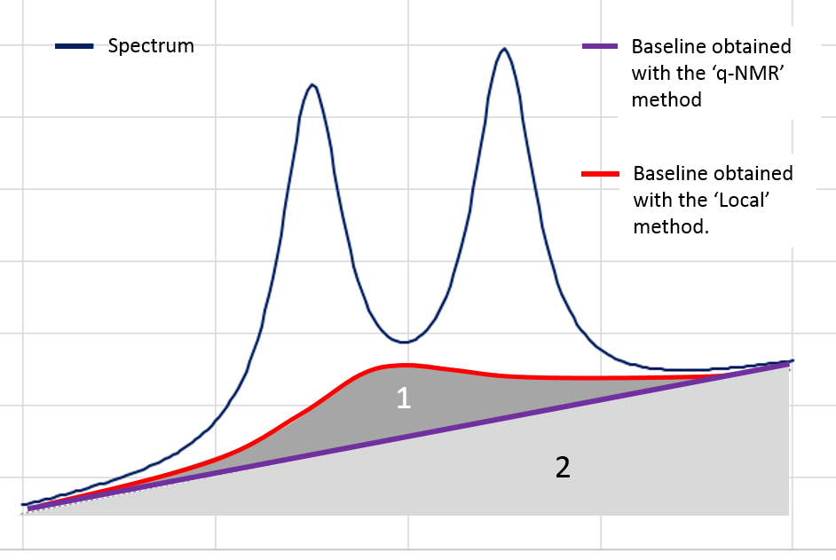
However, in the Targeted Metabolomics approach, a loss of "useful" variance even if it is slight cannot be tolerated; otherwise it also implies the loss of the 'absolute' feature of the quantification. In that case, the 'q-NMR' method is more relevant but it is to be applied to a small ppm range, i.e. a compound pattern (singlet, doublet or triplet).
References
Bao, Q., Feng, J., Chen, F., Mao, W., Liu, Z., Liu, K., et al. (2012).A new automatic baseline correction method based on iterative method. Journal of Magnetic Resonance, 218, 35–43. doi: 10.1016/j.jmr.2012.03.010.
Moing, A., Maucourt, M., Renaud, C., Gaudillere, M., Brouquisse, R., Lebouteiller, B., Gousset-Dupont, A., Vidal, J., Granot, D., Denoyes-Rothan, B., Lerceteau-Kohler, E., Rolin, D. (2004) Quantitative metabolic profiling by 1-dimensional H-1-NMR analyses: application to plant genetics and functional genomics. Functional Plant Biology 31, 889-902. doi: 10.1071/FP04066
Zhang Z, Chen S, and Liang Y-Z (2010) Baseline correction using adaptive iteratively reweighted penalized least squares, Analyst, 2010,135, 1138-1146. doi:10.1039/B922045C
Zheng, C., Zhang, S., Ragg, S., Raftery, D. and Vitek, O. (2011) Identification and quantification of metabolites in 1H NMR spectra by Bayesian model selection. Bioinformatics Vol. 27 (12) 1637:1644, doi:10.1093/bioinformatics/btr118

3 - Spectra alignment
The alignment step is undoubtedly one of the most tedious to solve. The misalignments are the results of changes in chemical shifts of NMR peaks largely due to differences in pH, ionic strength and other physicochemical interactions. To solve this prickly problem, we implemented three alignment methods, one based on a Least- Squares algorithm, one based on Cluster-based Peak Alignment and the other based on a Parametric Time Warping (PTW).
3.1 - Least- Squares algorithm for alignment
To align a set of spectra, we need to choose or to define a reference spectrum. The user can align spectra either based on a particular spectrum chosen within the spectra set, or based on the average spectrum. In this latter case, the re-alignment procedure is executed three times, the average spectrum being recalculated at each time.
In order to limit the relative ppm shift between the spectra to be realigned and the reference spectrum, the user can set this limit by adjusting the parameter 'Relative shift max.', that sets the maximum shift between spectra and the reference. The range goes from 0 (no ppm shift allowed) up to 1 (maximum ppm shift equal to 100% of the selected ppm range).
3.2 - Cluster-based Peak Alignment
A novel peak alignment algorithm, called hierarchical Cluster-based Peak Alignment (CluPA) is proposed by Vu et al (2011). The algorithm aligns a target spectrum to the reference spectrum in a top-down fashion by building a hierarchical cluster tree from peak lists of reference and target spectra and then dividing the spectra into smaller segments based on the most distant clusters of the tree. To reduce the computational time to estimate the spectral misalignment, the method makes use of Fast Fourier Transformation (FFT) cross-correlation.
3.3 - Parametric Time Warping for alignment
The implementation is based on the R package 'ptw' (Bloemberg et al. 2010). In this method, the spectra alignment consists in approximating the ‘time’ (ppm in our case) axis of the reference signal by applying a polynomial transformation of the ‘time’ (i.e. ppm) axis of the sample to be aligned.

where w() is the warping function. For more details, refer on the valuable explanations in Wehrens (2011).
Warnings: Wehrens R. (2011) highlights the fact that (§ 3.3.2) "alignment methods that are too flexible (such as PTW) may be led astray by the presence [so by the absence] of extra peaks, especially when these are of high intensity".
Note: In order to solve the different alignment cases, we have planned to include some other methods such as CluPA (Vu et al. 2013) or RUNAS (Alonso et al. 2014). We are currently testing these methods in order to evaluate their strengths and weaknesses compared to those we already implemented.
Which alignment method to choose?
Compliant with the NMRProcFlow philosophy and due to the diversity of problems encountered, for spectra alignment we chose the interactive approach. It means interval by interval, each interval being chosen by the user. We preconize to prioritize the CluPA method to align some large ppm areas (up to 2 or 3 ppm but no more). The larger the ppm zone, the higher the resolution should be. When the misalign zones are small, we recommand to choose the Least-Square method applied on spectra segments where intensities decrease to zero on both sides. It means that a baseline correction is also greatly preconized before attempting any alignment. Because the Least-Square method just applies a shift between spectra segments, this does not alter the lineshape of peaks. Regarding Targeted Metabolomics, this point is crucial for an absolute quantification. Nevertheless, when in presence of highly overlapped peaks and/or a highly misaligned zone, it could be valuable to apply the PTW method even if some peaks are altered in order to have at least an estimation, either of the concentration (Targeted Metabolomics) or of the relative integration value (Metabolic Fingerprinting).
References
Alonso, A., Rodríguez, M., Vinaixa, M., Tortosa, R., Correig, X., Julià, A., Marsal, S. (2014) Focus: a robust workflow for one-dimensional NMR spectral analysis. Anal Chem. 21;86(2):1160-9. doi: 10.1021/ac403110u
Bloemberg, T.G., Gerretzen, J., Wouters, H.J.P., Gloerich, J., van Dael, M., Wessels, H.J.C.T., et al. (2010). Improved parametric time warping for proteomics. Chemometrics and Intelligent Laboratory Systems, 104(1), 65-74. doi:10.1016/j.chemolab.2010.04.008
Vu T.N., Valkenborg D., Smets K., Verwaest K.A., Dommisse R., Lemière F., Verschoren A., Goethals B., Laukens K. An integrated workflow for robust alignment and simplified quantitative analysis of NMR spectrometry data. BMC Bioinformatics. 2011;12:405 doi: 10.1186/1471-2105-12-405
Wehrens R. (2011) Chemometrics with R: Multivariate Data Analysis in the Natural Sciences and Life Sciences, Ed Springer-Verlag Berlin Heidelberg doi: 10.1007/978-3-642-17841-2

4 - Binning
An NMR spectrum may contain several thousands of points, and therefore of variables. In order to reduce the data dimensionality binning or bucketing is commonly used. In binning, the spectra are divided into bins (so called buckets) and the total area (sum of each resonance intensity) within each bin is calculated to represent the original spectrum. The more simple approach (Uniform bucketing) consists in dividing all spectra with uniform spectral width (typically 0.01 to 0.04 ppm).
Due to the arbitrary division of spectrum, one bin may contain pieces from two or more resonances and one resonance may appear in two bins which may affect the data analysis. We have chosen to implement the Adaptive, Intelligent Binning method [De Meyer et al. 2008] that attempts to split the spectra so that each area common to all spectra contains the same single resonance, i.e. belonging to the same metabolite (Intelligent bucketing). In such methods, the width of each bucket is then determined by the maximum difference of chemical shifts among all spectra.

Such as AIBIN method, a method called ERVA (Extraction of Relevant Variables for Analysis) (Jacob et al, 2013) attempts to split the spectra so that each area common to all spectra contains the same single resonance, i.e. belonging to the same metabolite. This mathematical method is based on a convolution product between a spectrum (S) and the second-order derivative of the Lorentzian function (SDL). This products buckets that are exactly centered on each resonance having their width equal to twice the half-width of the resonance.

Another way for obtaining buckets is to choose the ppm ranges the user wants to integrate (Variable size bucketing). This method is typically used for the Targeted Metabolomics approach where only few resonances corresponding to targeted compounds are selected with their size depending on the signal pattern.
Note: The novel binning method called ERVA (Extraction of Relevant Variables for Analysis) will be soon available within NMRProcFlow, which that will greatly help the identification task of potential biomarker. (Jacob et al 2013) - See presentation online for more details on this approach.
Which binning method to choose?
Regarding the Targeted Metabolomics approach, clearly the ‘Variable size bucketing’ has to be chosen for reasons given above. Regarding the Metabolic Fingerprinting approach, the choice is depending if the alignment has been done or not. If yes and even in a imperfect way, the Intelligent bucketing or the ERVA method are clearly the most efficient. In case the alignment remains a too tedious task to be accomplished, one can choose the uniform bucketing as the most fast and simple (given that 'intelligence' will change nothing in the matter). But in this latter case, we strongly recommend after any subsequent statistical analyses to check the quality of the buckets especially those highlighted from Discriminant Analysis (e.g PLS-DA, OSC-PLS-DA ...). This has to be done with a critical eye by visualizing the overlaid spectra for these buckets, and thus ensuring that it is not due to a local misalignment.
References
De Meyer, T., Sinnaeve, D., Van Gasse, B., Tsiporkova, E., Rietzschel, E. R., De Buyzere, M. L., et al. (2008). NMR-based characterization of metabolic alterations in hypertension using an adaptive, intelligent binning algorithm. Analytical Chemistry, 80(10), 3783–3790.doi: 10.1021/ac7025964
Jacob D., Deborde C. and Moing A. (2013). An efficient spectra processing method for metabolite identification from 1H-NMR metabolomics data. Analytical and Bioanalytical Chemistry 405(15) 5049–5061 doi: 10.1007/s00216-013-6852-y

5 - Buckets integration
The integration of buckets or zones of interest for targeted analysis is carried out according to the traditional trapezoid method. Knowing that a NMR spectrum is discretized at constant step, the formula is straightforward and described as follows.
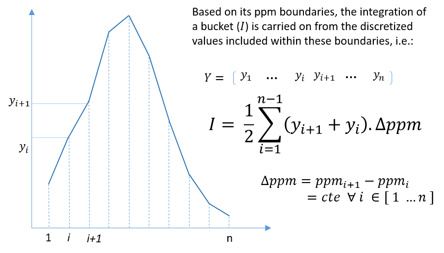
6 - Bucket normalization
Before bucket data export, in order to make all spectra comparable with each other, the variations of the overall concentrations of samples have to be taken into account. We propose three normalization methods. In NMR metabolomics, the total intensity normalization (called the Constant Sum Normalization) is often used so that all spectra correspond to the same overall concentration. It simply consists in normalizing the total intensity of each individual spectrum to a same value.
Other methods such as Probabilistic Quotient Normalization [Dieterle et al. 2006] assume that biologically interesting concentration changes influence only parts of the NMR spectrum, while dilution effects will affect all metabolite signals. Probabilistic Quotient Normalization (PQN) starts by the calculation of a reference spectrum based on the median spectrum. Next, for each variable of interest the quotient of a given test spectrum and reference spectrum is calculated and the median of all quotients is estimated. Finally, all variables of the test spectrum are divided by the median quotient. An internal reference can be used to normalize the data. For example, an electronic reference (ERETIC, (see Akoka et al. 1999), or ERETIC2 generated with TopSpin software) can be used for this purpose. The integral value of each bucket will be divided by the integral value of the ppm range given as reference.
Which normalization method to choose?
We suggest the reference [Kohl et al. 2012] as a good review that could be read with great profit.
References
Akoka S1, Barantin L, Trierweiler M. (1999) Concentration Measurement by Proton NMR Using the ERETIC Method, Anal. Chem 71(13):2554-7. doi: 10.1021/ac981422i.
Dieterle F., Ross A., Schlotterbeck G. and Senn H. (2006). Probabilistic Quotient Normalization as Robust Method to Account for Dilution of Complex Biological Mixtures. Application in 1H NMR Metabonomics. Analytical Chemistry, 78:4281-4290.doi: 10.1021/ac051632c
Kohl SM, Klein MS, Hochrein J, Oefner PJ, Spang R, Gronwald W. (2012) State-of-the art data normalization methods improve NMR-based metabolomic analysis, Metabolomics 146-160, doi: 10.1007/s11306-011-0350-z

Data preparation phase
The current version of NMRProcFlow accepts raw data come from four major vendors namely Bruker GmbH, Agilent Technologies (Varian), Jeol Ltd and RS2D. Moreover, we also support the nmrML format (See nmrml.org for further information on this format)
Regarding Bruker, two types of raw data are accepted: Free Induction Decay (fid) and pre-processed raw spectra (1r). In both cases, the folder structure must follow that of the Bruker TopSpin software. "Pre-processed" means that it assumes that Fourier transform and phase correction have been applied on all spectra so that their corresponding processing directory (under 'pdata') exists along with their real spectrum (i.e 1r file). In the case where the input raw data are FID, the spectral pre-processing is automatically performed. See the Spectral pre-processing for 1D NMR section.
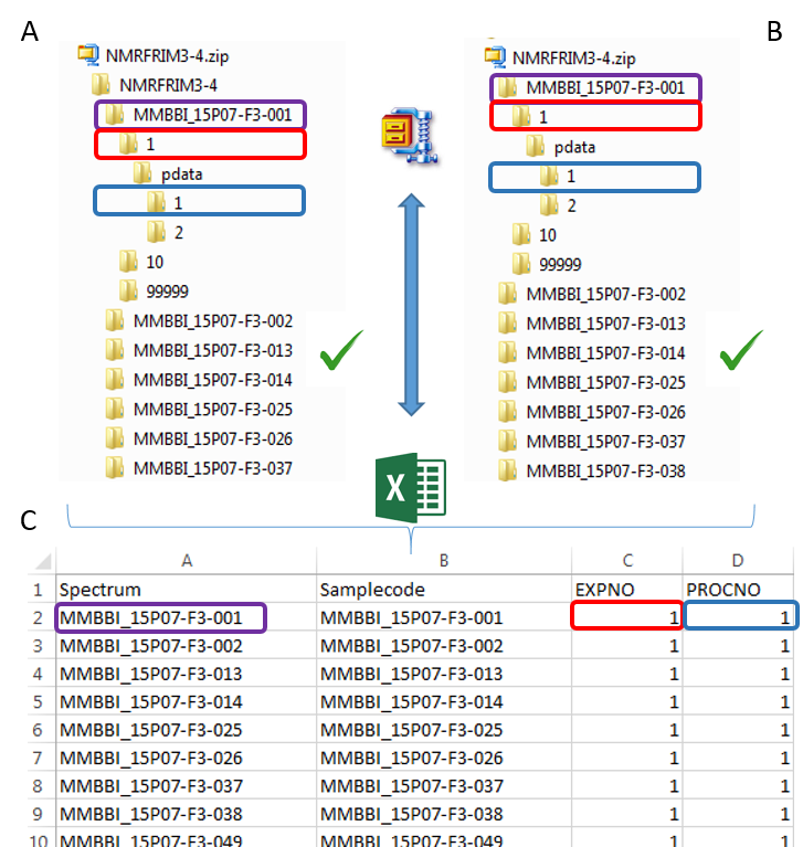
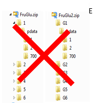
To ease the preparation phase, simply zip the entire directory including all spectra of the experiment. This means that it is useless to perform any prior selection or having to rename the numbers of experiment and processing. The figure below shows an example of ZIP file along with its corresponding samples file.
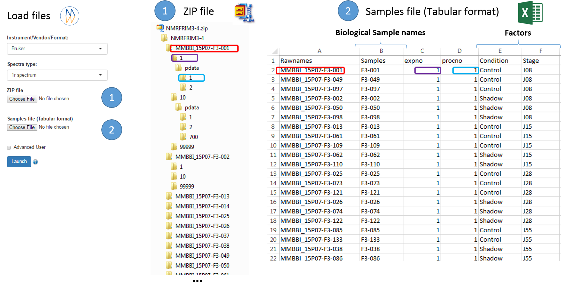
The colored boxes show the correspondences.
Supported directory structures for Bruker NMR spectra
Information provided within the samples file must correspond to the directories contained in the ZIP file. (The colored boxes show the correspondences)
- The 'rawdata' column may include all directories or just a subset contained in the ZIP file.
- The 'Samplecode' column can be filled with the biological sample name or can be just a copy-paste of the 'Rawdata' column.
- The 'expno' and 'procno' columns correspond to the experiment number (i.e. FID) and the processing number (i.e. 1r) respectively.
- Several factor columns can be added which will allow spectra to be visualized according to theirs factor levels (see example online). The only constraints on factor names are that they must be alphanumeric characters [0..9, a..z, A..Z]. The underscore '_' is also allowed.
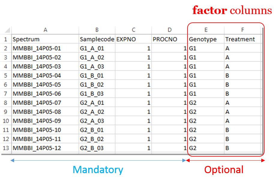
In this way, it becomes easy to select each NMR spectrum that we want to include into the spectra serial in order to be processed together. In the absence of the file of samples provided as an input, NMRProcFlow will consider all of the root directories in the zip file by default, looking for the smallest FID identifier (expno) and the smallest processing identifier (procno) for each of them.
Warnings: In the case where the input raw data are FID, the 'procno' column has to be kept (e.g. filled with zero) so that the samples file is thus compliant with both type of input data (fid & 1r)
To facilitate the generation of the samples file, it is possible to proceed as follows:
- Upload the ZIP file only, and then NMRProcFlow will produce a text file containing the acquisition and processing parameters for each spectrum taken into account by default,
- Download the parameters file ('Export Parameters'),
- Edit this file to serve as a starting template for generating the samples file.
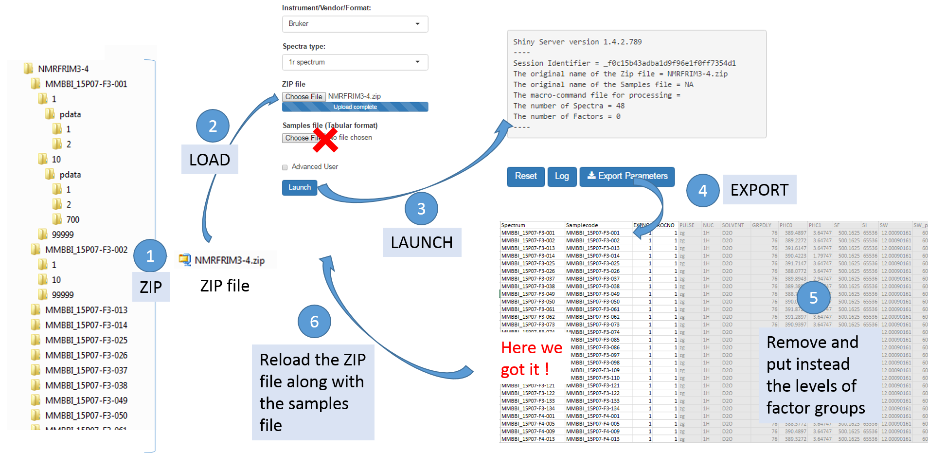
Once uploaded files, you can click on 'Launch' to start the pretreatment.
Once completed, the list of spectra considered with their acquisition and pre-processing parameters is provided
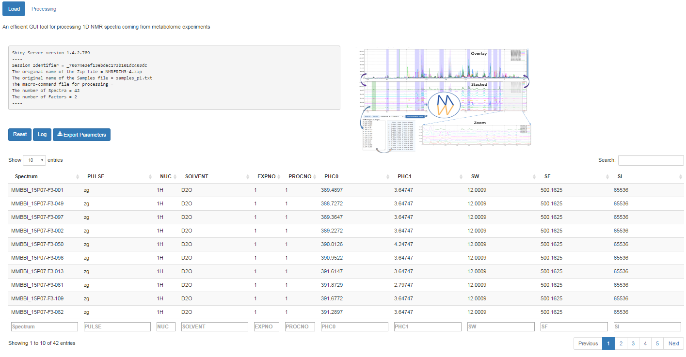
To switch to the processing steps, you must click on the 'Processing' tab at the top of the screen.

Regarding Agigent/Varian, only the Free Induction Delay are accepted, given that there is no normalized folder structure for pre-processed raw data provided by the OpenVnmrJ software. See the Spectral pre-processing for 1D NMR section to know how to choose parameters.
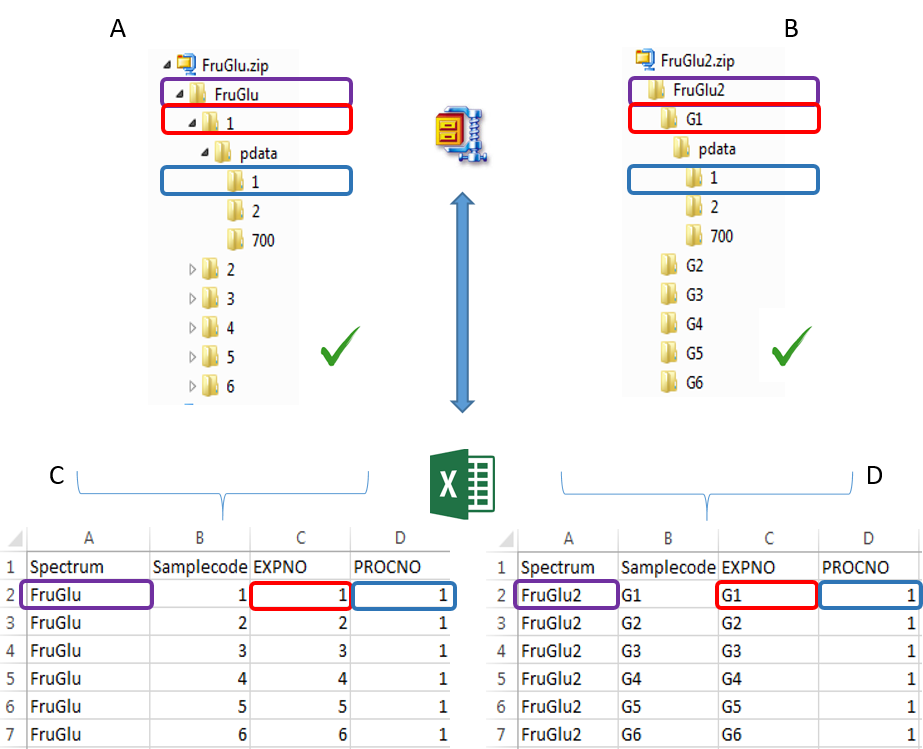
To ease the preparation phase, simply zip the entire directory including all spectra of the experiment. This means that it is useless to perform any prior selection or having to rename the numbers of experiment and processing. The figure below shows an example of ZIP file along with its corresponding samples file.
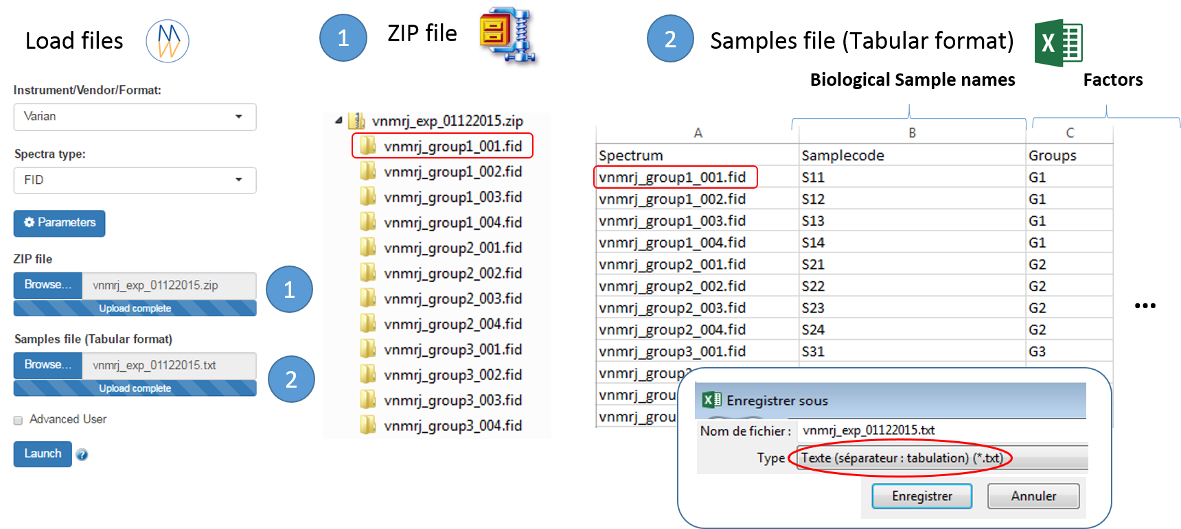
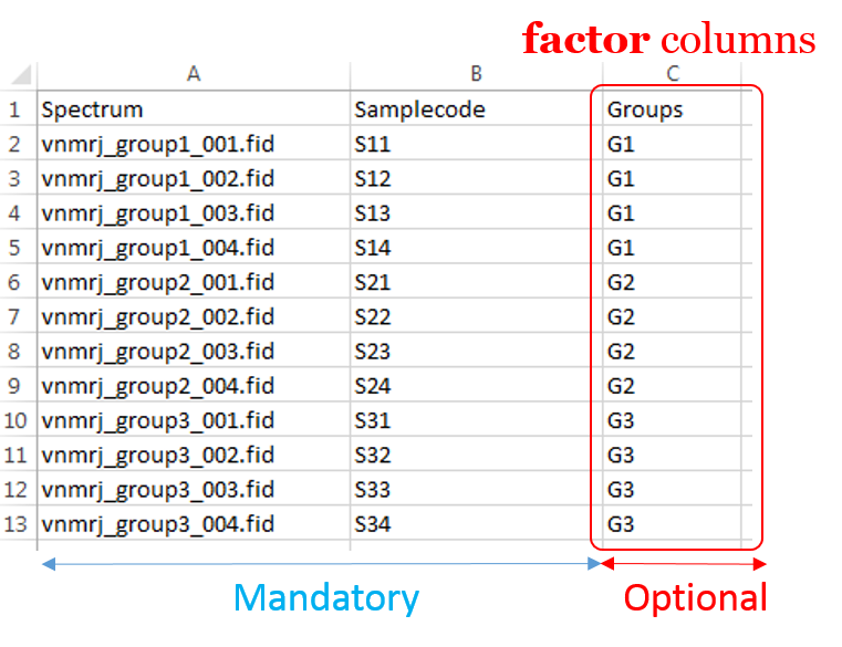
Information provided within the samples file must correspond to the directories contained in the ZIP file. (The colored boxes show the correspondences)
- The 'rawdata' column may include all directories or just a subset contained in the ZIP file.
- The 'Samplecode' column can be filled with the biological sample name or can be just a copy-paste of the 'Rawdata' column.
- Several factor columns can be added which will allow spectra to be visualized according to theirs factor levels. The only constraints on factor names are that they must be alphanumeric characters [0..9, a..z, A..Z]. The underscore '_' is also allowed.
In this way, it becomes easy to select each NMR spectrum that we want to include into the spectra serial in order to be processed together. In the absence of the file of samples provided as an input, NMRProcFlow will consider all of the root directories in the zip file by default, looking for all FID files.
To facilitate the generation of the samples file, see the corresponding section in the 'Bruker' tab
Once uploaded files, you can click on 'Launch' to start the pretreatment.
Once completed, the list of spectra considered with their acquisition and pre-processing parameters is provided
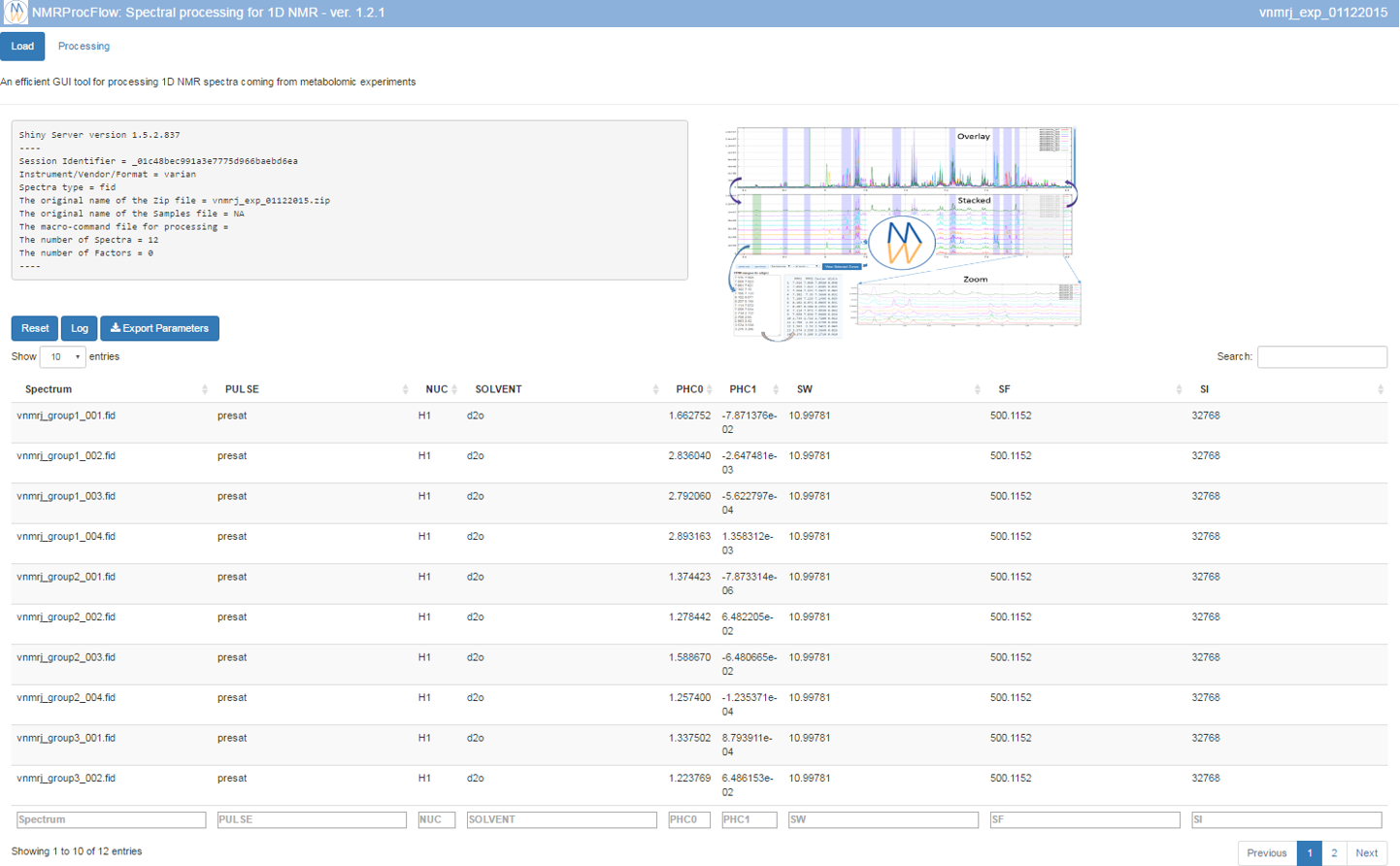
To switch to the processing steps, you must click on the 'Processing' tab at the top of the screen.

Since March 2018, the NMR Jeol spectra are supported (only the Free Induction Delay) within the JDF format created from the Jeol Delta software.
- See the Spectral pre-processing for 1D NMR section.
- See a complete example with a JEOL spectra set (JDF Format) - (PDF online)
Since March 2019, the NMR RS2D spectra are supported (both Free Induction Delay and Spectrum in frequency domain) within the SPINit format created from the SPINit software.
- See the Spectral pre-processing for 1D NMR section.
- See a complete example with a RS2D spectra set (SPINit Format) - (PDF online)
Since January 2018, the nmrML format are supported (only the Free Induction Delay).
- See the Spectral pre-processing for 1D NMR section.
- See an example of nmrML convertion of a JEOL spectra set (JDF Format) before uploading within NMRProcFlow - (PDF online)
References
Schober D, Jacob D, Wilson M, Cruz JA, Marcu A, Grant JR, Moing A, Deborde C, de Figueiredo LF, Haug K, Rocca-Serra P, Easton J, Ebbels TMD, Hao J, Ludwig C, Günther UL, Rosato A, Klein MS, Lewis IA, Luchinat C, Jones AR, Grauslys A, Larralde M, Yokochi M, Kobayashi N, Porzel A, Griffin JL, Viant MR, Wishart DS, Steinbeck C, Salek RM, Neumann S. (2018) Anal Chem doi: 10.1021/acs.analchem.7b02795

Spectral pre-processing for 1D NMR
The spectral preprocessing for 1D NMR (1H & 13C) can be automatically applied in case where the input raw data are FID. The term pre-processing designates here the transformation of the NMR spectrum from time domain to frequency domain, including the phase correction and the fast fourier-transform (FFT).(For more details, see Processing methods)
Here, we suggest a reference that could be read with great profit:
James Keeler (2010) Understanding NMR Spectroscopy, 2nd Edition, Ed Wiley
In NMRProcFlow, you can adjust some parameters. Just click on the 'Parameters' button to bring up the window of the parameters to be adjusted, as shown bellow:
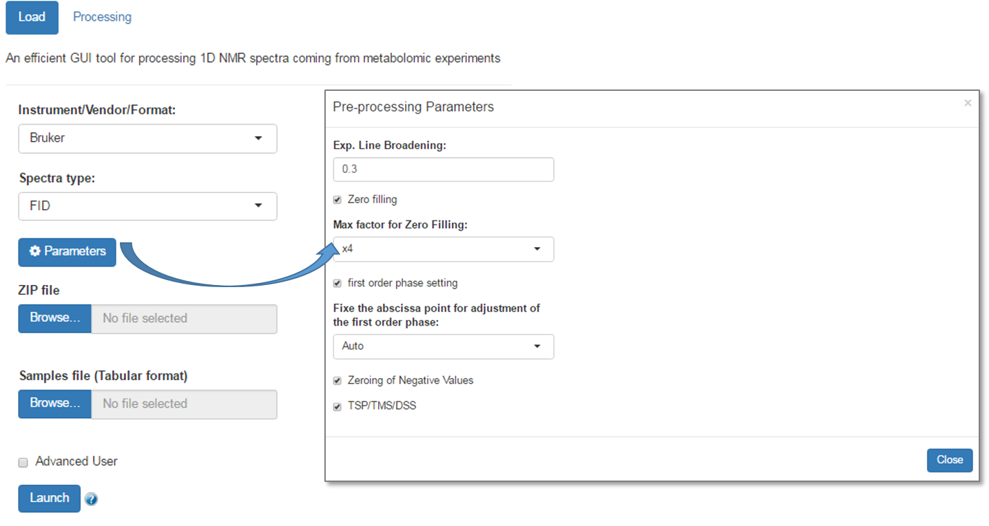
- Line Broadening: Apodization is based on a Line Broadening (i.e an exponential) applied on the fid in order to improve the signal-noise ratio. You can modify the parameter (LB). Zero means no apodization. If necessary, by playing very slightly on the LB parameter, sometimes this may greatly improve the phase correction. Warning: higher the LB value, poorer the resolution.
- Zero filling: This consists of adding zeros at the end of the FID signal such as the resulting size is an even multiple of the initial size. Contrary of an apodization, this has less effect on the spectra resolution, while improving the signal-to-noise ratio.
- First order phase can be adjusted (by default) or not. In case of the First order phase needs to be adjusted, the abscissa point (α) used to set the first order phase can be automatically fixed, otherwise you can choose a value in the dropbox list.
Note: You can optimize the parameters to apply on your own raw spectra from the small application online at the URL https://pmb-bordeaux.fr/nmrspec/.

View the spectra
The NMR spectra viewer is the central tool of NMRProcFlow and the core of the application. It allows the user:
- To visually explore the spectra either overlaid or stacked,
- To zoom in for intensity and/or ppm scales,
- To color each subset of spectra according to their corresponding factor levels
- To capture a ppm range using the mouse to stick it in the suitable input box in order to process this ppm range
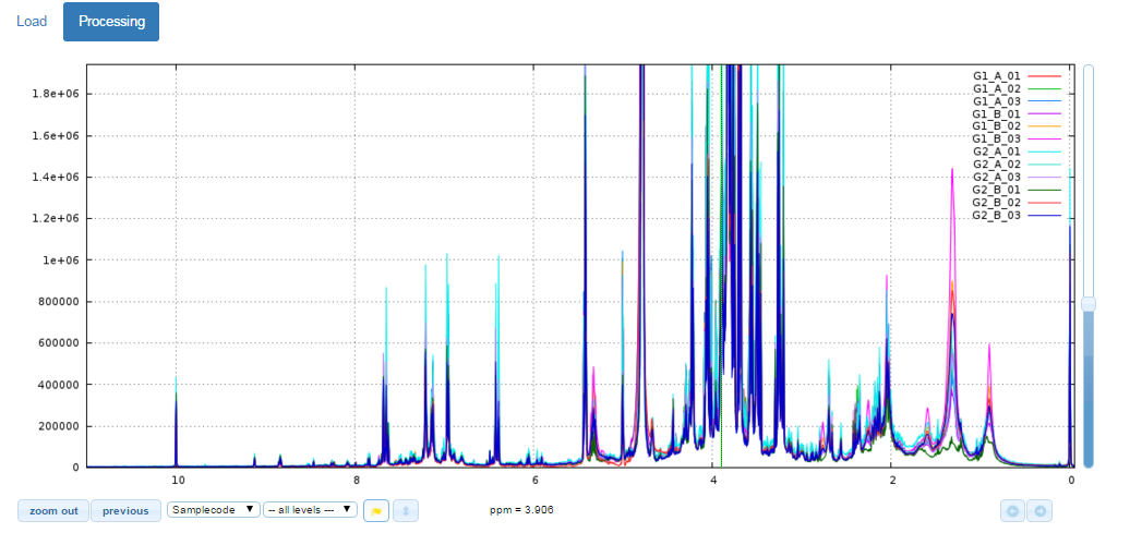
Test online the NMR Spectra Viewer
Because the NMR spectra viewer is the central tool of NMRProcFlow it occupies more than half of the window.
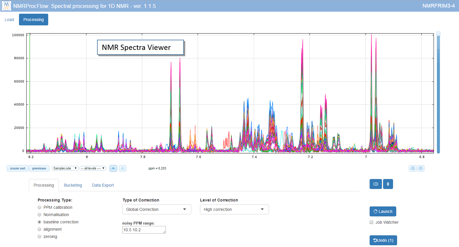
Tip: For a better view and according to your screen resolution, think about slightly reduce the zoom of your web browser (e.g. 90%)
Overlay / Stack and Spectra Colors

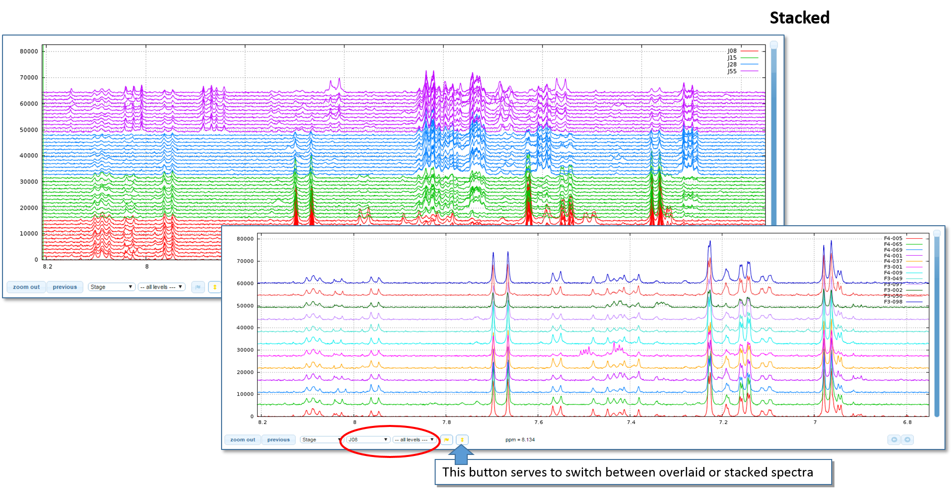
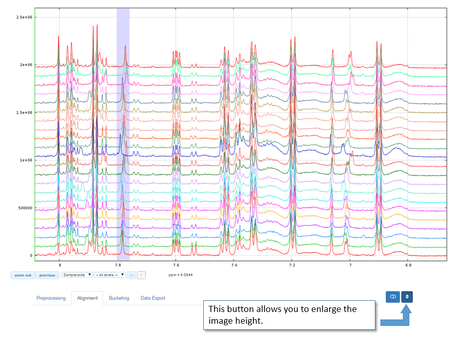
Enlarge the image height

Interactive data processing
It is possible to navigate between tabs and then launch any processing in the order you want.
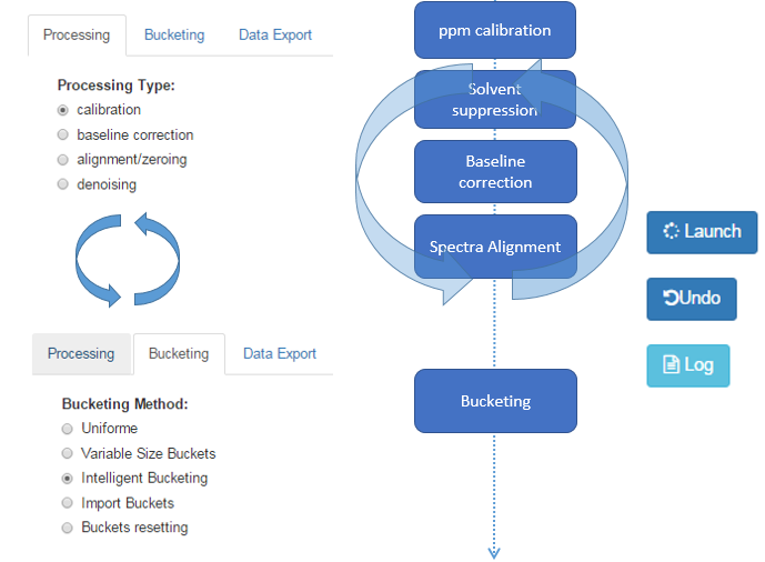
In addition, it is possible to cancel each treatment performed in the order in which it was made. The ‘Undo’ button gives the count of performed processing and that can therefore be cancelled.
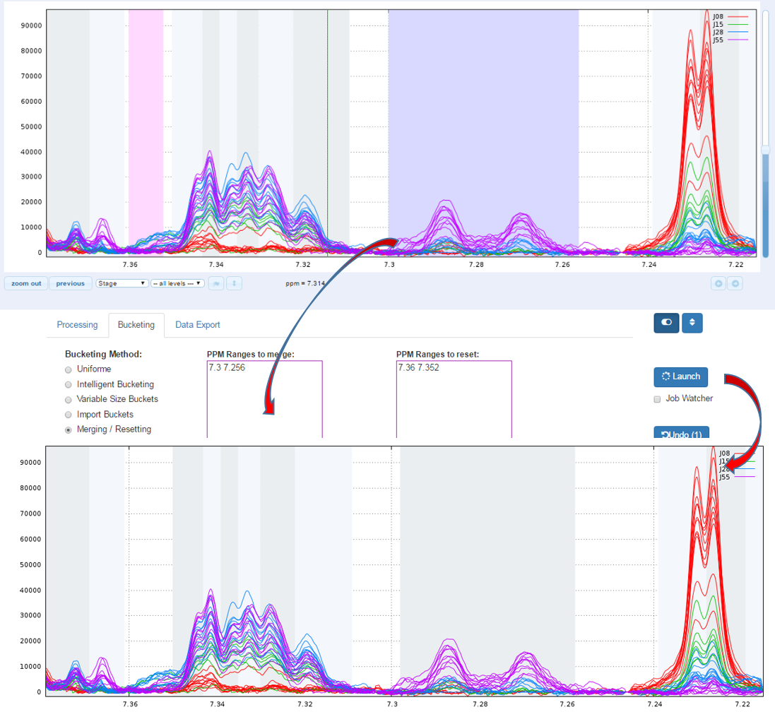
However, the bucketing processing can be launched and cancelled independently of those performed through the ‘processing’ tab. Indeed, in the latter case, the different kinds of processing involve modifying the spectra themselves, while the bucketing only adds an information layer (the zone of each bucket). A good practice is to launch a bucketing in order to see what the problematic zones are (typically the misalignments). After solving these ones, a bucketing can be launched again in order to see if the problem was correctly solved. If not, the previous processing can be cancelled and replayed with other parameters.
Interaction with the spectra viewer
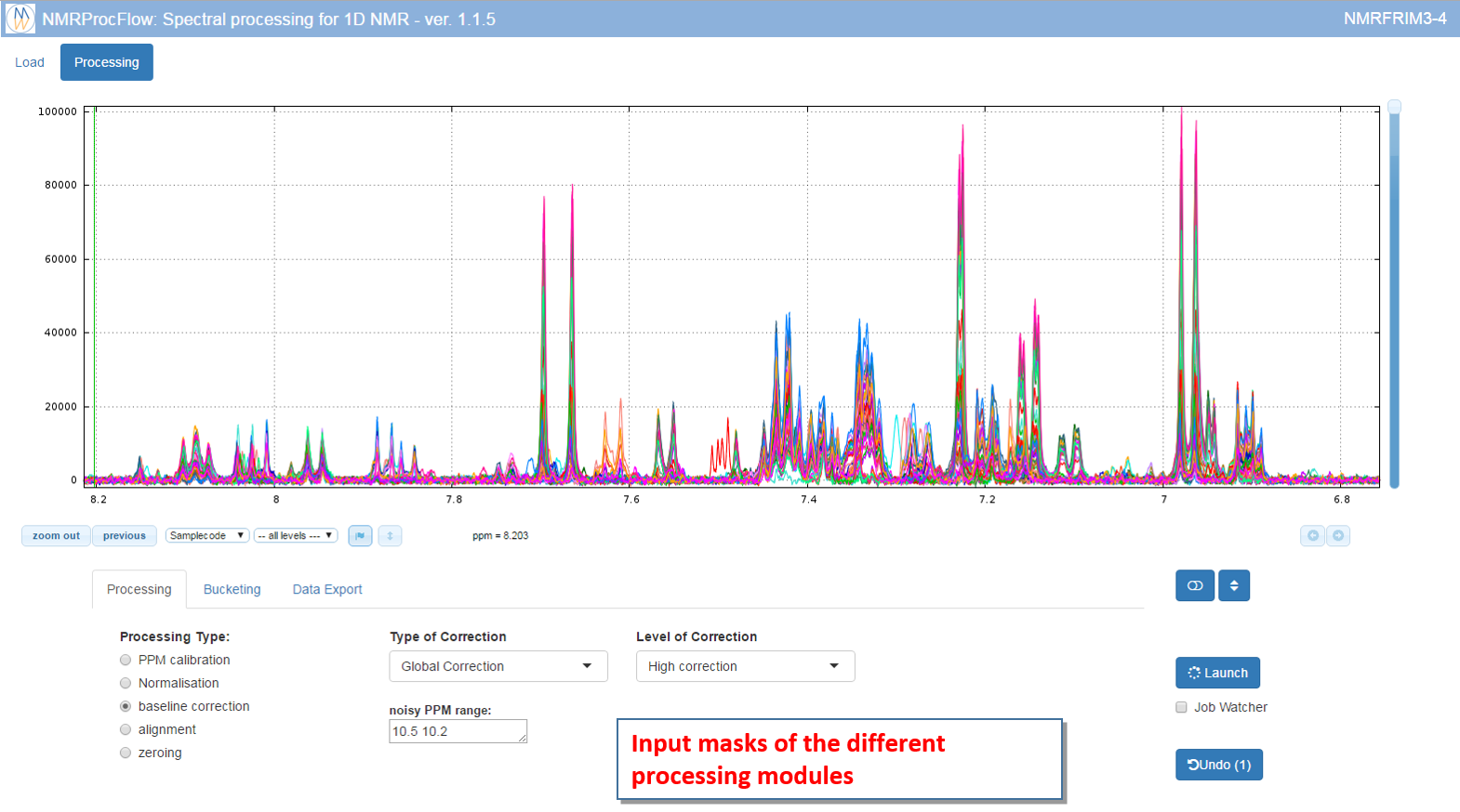
The processing panel is organized into two distinct areas: 1) the NMR spectra viewer at the top, and 2) the input masks of the different processing modules
How to capture a ppm range within a box?
A ppm range can be captured using the mouse to stick it in the suitable input box in order to process this ppm range
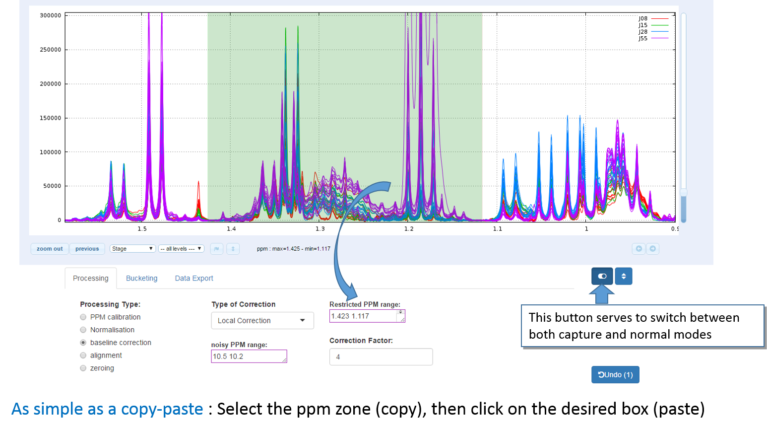
To select a ppm range:
- Toggle into 'capture' mode, then press down the left mouse button at the start of the range, then move the mouse up to the end of the range, then release the mouse button.
- Click on the textbox corresponding to the type of process you want to apply to this range. Textboxes that accept such ppm range capture have a purple outline.
Note: Instead of using the switch button, another way is to press down one of both 'Ctrl' or 'Alt' keys and maintain it down while you copy-paste the ppm zone, then release the key up.
How to capture / save images of the NMR spectra on your disk space ?
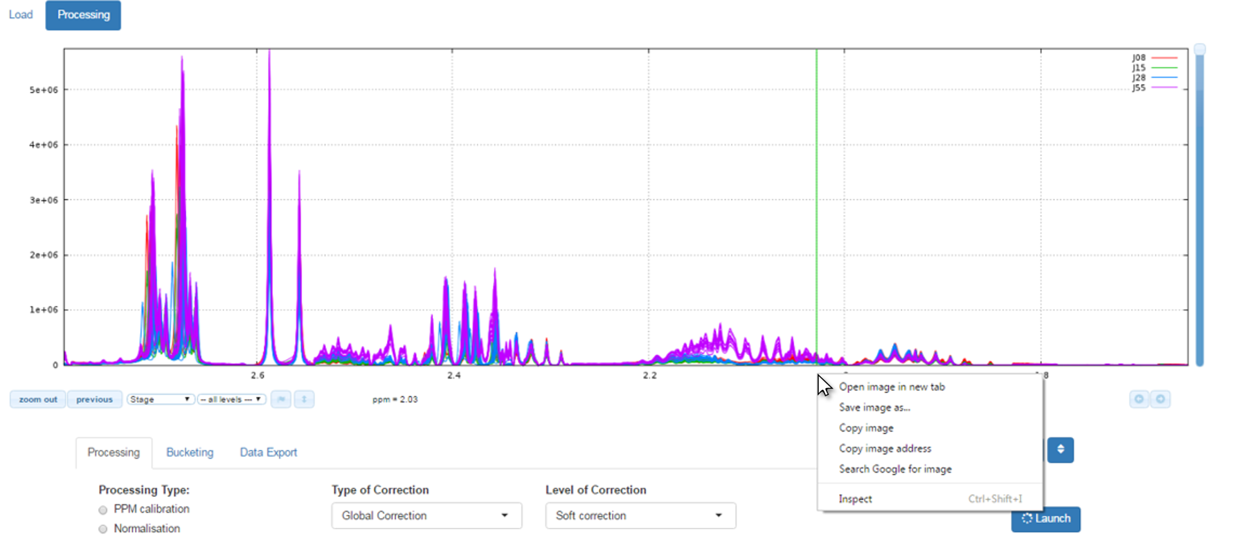
Simply by clicking on the right button of your mouse just on the spectra viewer (preferably at the ppm graduations) and the context menu appear, as shown below:

Spectra processing
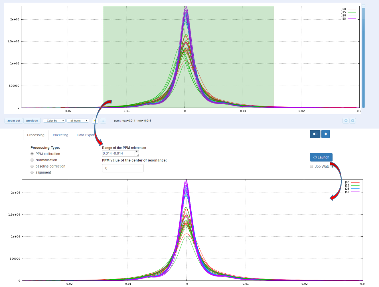
The calibration of the scale of PPM is to adjust the chemical shifts according to a known reference. The reference compound used for chemical shift (δ=0.00) is usually the sodium salt of 3-trimethylsilylpropionic acid-d4 (TSP-d4) with deuterated methylene groups. Other references standards are 2,2- 23 dimethyl-2-silapentane-5-sulfonate sodium salt (DSS) or for organic solvent trimethylsilane (TMS). But it may be any other compound such as creatinine (4.06ppm), α-glucose (5.23ppm), alanine (a doublet along with a peak at 1.488ppm), etc...
How to proceed (see fig below)
- Capture the reference peak into the ‘Range of the PPM reference’ box
- Specify the ppm value corresponding to the highest intensity of the reference peak
- Then launch

Because on the one hand the peak integration is very sensitive to baseline distortions and on the other hand the baseline distortions may not affect in the same way each spectrum, we have to apply a baseline correction.
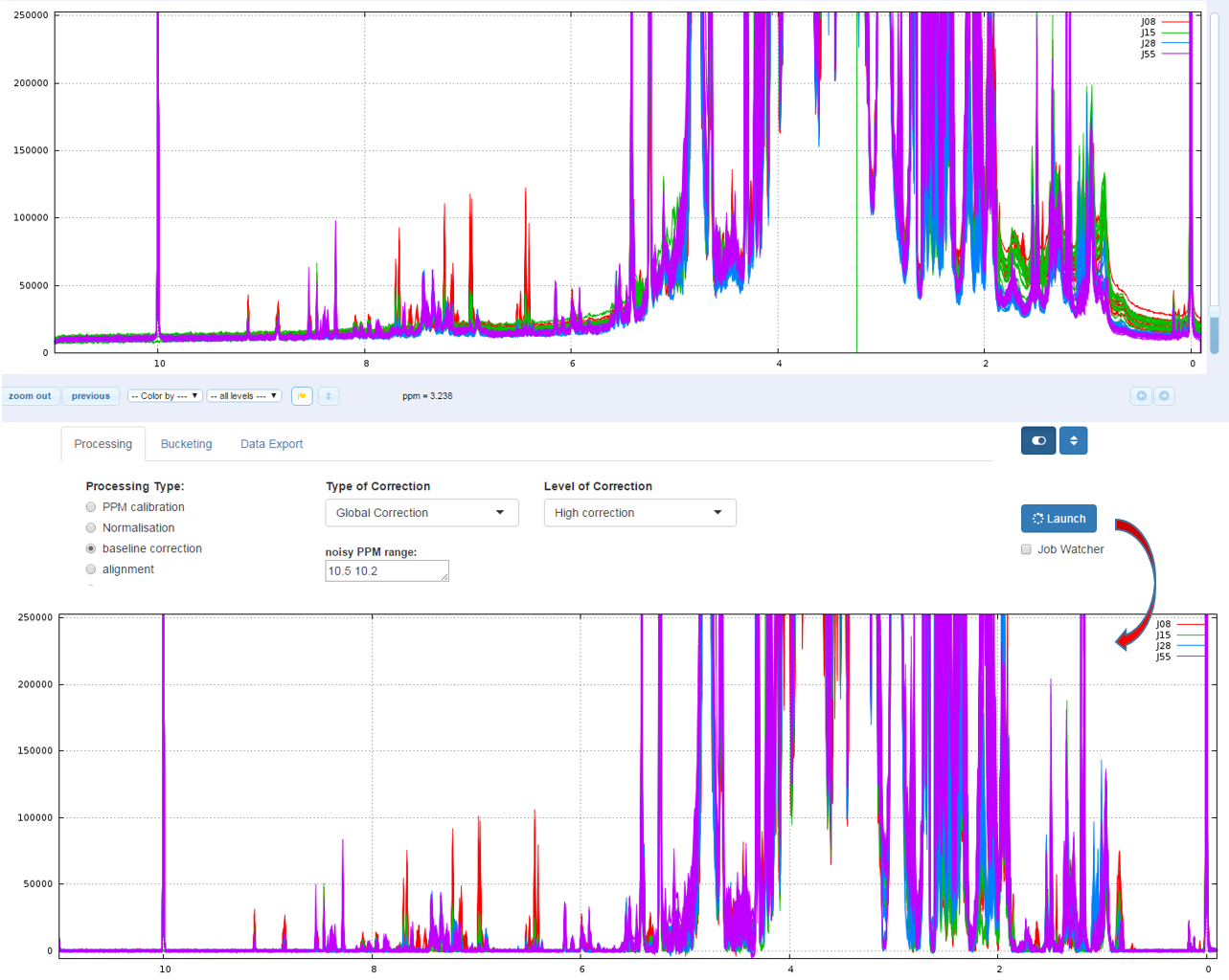
Two types of Baseline correction were implemented: Global and Local. (For more details, see Processing methods). To be more efficient, both methods need to estimate the noise level, and by default the ppm range included between 10.2 and 10.5 ppm is taken. But you can choose another one if some signal is present in this area.
1 - Global
The global baseline correction was based on [Bao et al, 2012], but only two phases were implemented: i) Continuous Wavelet Transform (CWT) and ii) the sliding window algorithm. The user must choose the correction level, from 'soft' up to 'high'.
How to proceed (see fig below)
- Choose the correction level, from 'Soft correction' up to 'High correction'
- Capture the ppm range in order to estimate the noise level
- Then launch
Bao et al (2012) A new baseline correction method based on iterative method, Journal of Magnetic Resonance 218 (2012) 35-43
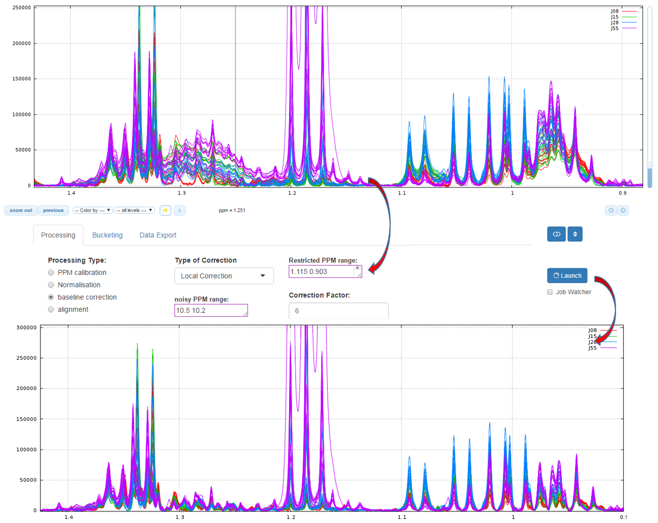
2 - Local
The airPLS (adaptive iteratively reweighted penalized least squares) algorithm based on [Zhang et al, 2010] is a baseline correction algorithm which works completely on its own, and that does only require a detail parameter for the algorithm, called Lambda. Because this Lambda parameter can vary within a very large range (from 10 up to 1.e+06), we converted this parameter within a more convenient scale for the user, called 'level correction factor' chosen by the user from '1' (soft) up to '6' (high). The lower this level correction factor is set the smoother baseline will be. Conversely, the higher this level correction factor is set, the more baseline will be corrected in details. To be more efficient, the algorithm needs to estimate the noise level, and it takes by default the ppm range included between 10.2 and 10.5 ppm. But you can choose another one if some signal is present in this area
How to proceed (see fig below)
- Capture the ‘Range of the PPM’ to be corrected
- Choose the correction level, from '1' up to '7'
- Capture the ppm range in order to estimate the noise level
- Then launch
Zhang Z, Chen S, and Liang Y-Z (2010) Baseline correction using adaptive iteratively reweighted penalized least squares, Analyst, 2010,135, 1138-1146. doi:10.1039/B922045C
The alignment step is undoubtedly one of the most tedious to solve. The misalignments are the results of changes in chemical shifts of NMR peaks largely due to differences in pH and other physicochemical interactions. To solve this prickly problem, we implement two alignment methods, one based on a Least- Squares algorithm and the other based on a Parametric Time Warping (PTW). Compliant with the NMRProcFlow philosophy and due to the diversity of problems encountered we chose for spectra alignment, the interactive approach. It means interval by interval, each interval being chosen by the user. (For more details, see Processing methods)
1 - Least- Squares algorithm
To align a set of spectra, we need to choose or to define a reference spectrum. You can align spectra either based on a particular spectrum chosen within the spectra set, or based on the average spectrum. In this latter case, the re-alignment procedure is executed three times, the average spectrum being recalculated at each time
In order to limit the relative ppm shift between the spectra to be realigned and the reference spectrum, you can set this limit by adjusting the parameter 'Relative shift max.', that sets the maximum shift between spectra and the reference. The range goes from 0 (no ppm shift allowed) up to 1 (maximum ppm shift equal to 100% of the selected ppm range)
1.1 - How to proceed (see fig below)
- Capture the ‘Range of the PPM’ to be aligned
- Set the 'Relative max/ shift'
- Choose the 'Reference Spectrum'
- Then launch
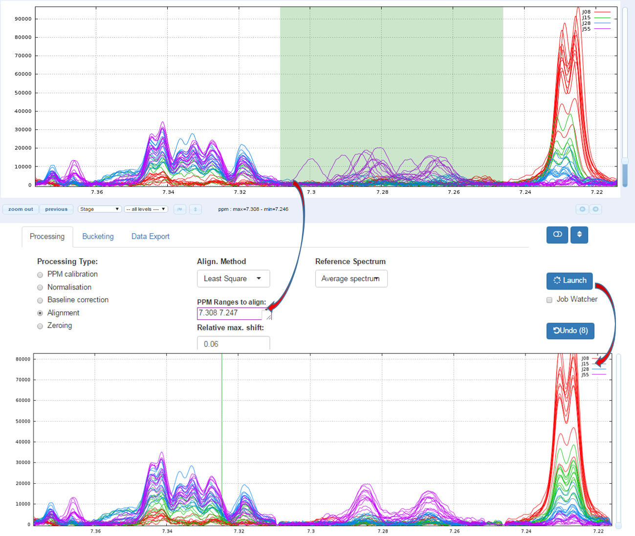
1.2 - Example showing the importance of the "Relative max. shift" parameter (see fig below)
Consider that we want to align spectra within the ppm range defined by the window as shown below:

With no way to limit the shifts between spectra, (ie. this corresponds to a relative maximum shift equal to 100%), we have the following result:

Clearly, it is not the right result. So, we set now a relative maximum shift equal to 5% (ie 0.05), and we have the right result, as shown below:

2 - Parametric Time Warping
The modus operandi for this method is very similar to the previous one, apart the "Relative max. shift" parameter that is not needed. The implementation is based on the R package 'ptw' (Bloemberg et al. 2010) and on the valuable explanations in Wehrens R. (2011).
2.1 - Example of comparison between the Least-Square and PTW methods (see fig below)
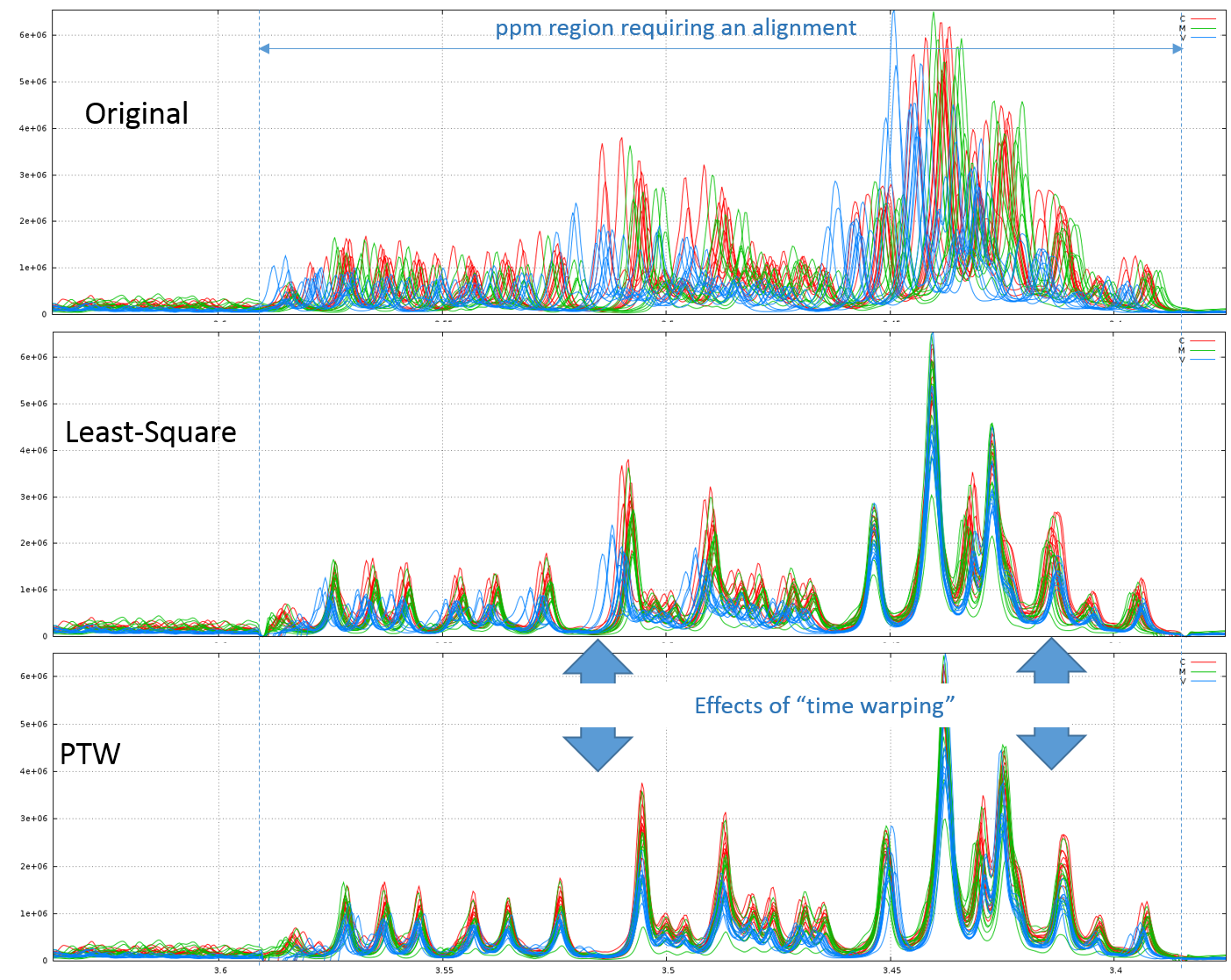
Clearly, in this example, PTW method is more efficient than a simple Least-Square approach.
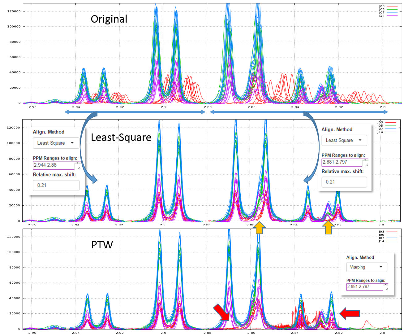
Warnings: Wehrens R. (2011) highlights the fact that (§ 3.3.2) "alignment methods that are too flexible (such as PTW) may be led astray by the presence [so by the absence] of extra peaks, especially when these are of high intensity". Therefore, a "very esthetic alignment" must not be the only quality criterion.
A good example is shown in the figure below. We first align the spectra in two steps using the Least-Square approach. The orange arrows show the absence of one peak for one stage (J03). Then, we undo the second alignment of the zone that included the problematic peak and we align again this zone using the PTW approach. All spectra are seem well-aligned apart those corresponding to the J03 stage. The red arrows show the zones where the PTW algorithm has been "astray".
T.G. Bloemberg, J. Gerretzen, H.J.P. Wouters, J. Gloerich, M. van Dael, H.J.C.T. Wessels, L.P. van den Heuvel, P.H.C. Eilers, L.M.C. Buydens, and R. Wehrens. Improved parametric time warping for proteomics. Chemom. Intell. Lab. Systems, 2010.
Wehrens R. (2011) Chemometrics with R: Multivariate Data Analysis in the Natural Sciences and Life Sciences, Ed Springer-Verlag Berlin Heidelberg

Bucketing
An NMR spectrum may contain several thousands of points, and therefore of variables. In order to reduce the data dimensionality binning is commonly used. In binning the spectra are divided into bins (so called buckets) and the total area within each bin is calculated to represent the original spectrum. The more simple approach consists to divide all the spectra with uniform areas width (typically 0.04 ppm). Due to the arbitrary division of peaks, one bin may contain pieces from two or more peaks which may affect the data analysis. We have chosen to implement the Adaptive, Intelligent Binning method [De Meyer et al. 2008] that attempt to split the spectra so that each area common to all spectra contains the same resonance, i.e. belonging to the same metabolite. In such methods, the width of each area is then determined by the maximum difference of chemical shift among all spectra.
How to proceed (see fig below)
- Specify a relevant zone in order to estimate the noise level.
- Choose a resolution factor between 0.1 and 0.6 (0.5 is the default value); the smaller value the greater resolution
- Select one or more PPM zones for applying the binning and put them in the box of ‘PPM ranges’
- Choose the threshold of the Signal/Noise Ratio (SNR) so that the buckets having a lower average integration will be excluded.
- Then launch
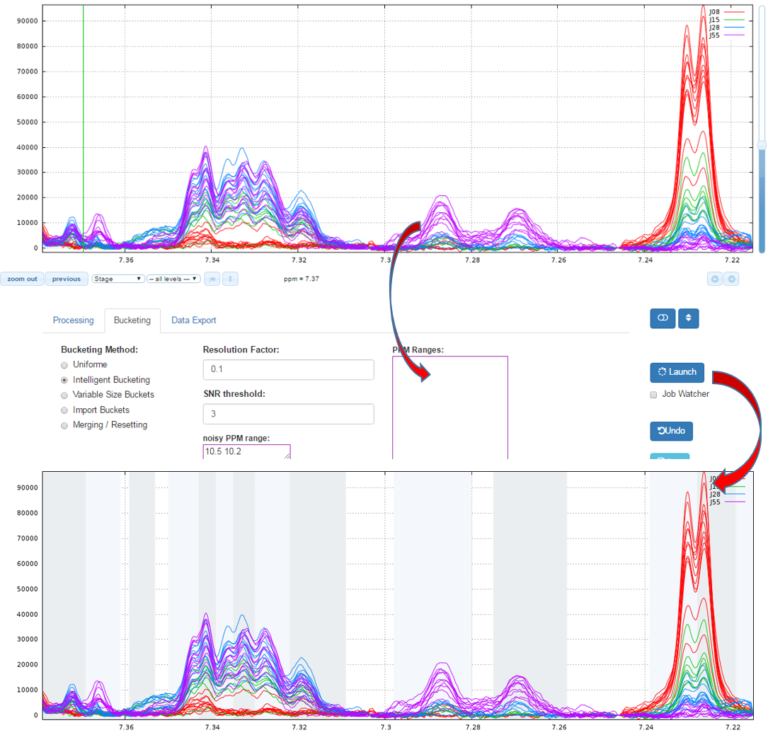
Warnings:Do not choose a resolution parameter too small in an area where alignment has not been made. NMRProcFlow makes it possible to adapt area by area the right resolution.
de Meyer T, Sinnaeve D, van Gasse B, Tsiporkova E, Rietzschel E, de Buyzere M, Gillebert T, Bekaert S, Martins J, van Criekinge W (2008) NMR-based characterization of metabolic alterations in hypertension using an adaptive, intelligent binning algorithm. Anal Chem 80:3783–3790

Another way for obtain buckets is to choose yourself ppm ranges you want to integrate. This method is typically used for the Targeted metabolomics approach where only few peaks corresponding to targeted compounds are selected whose their size is depending of the signal pattern.
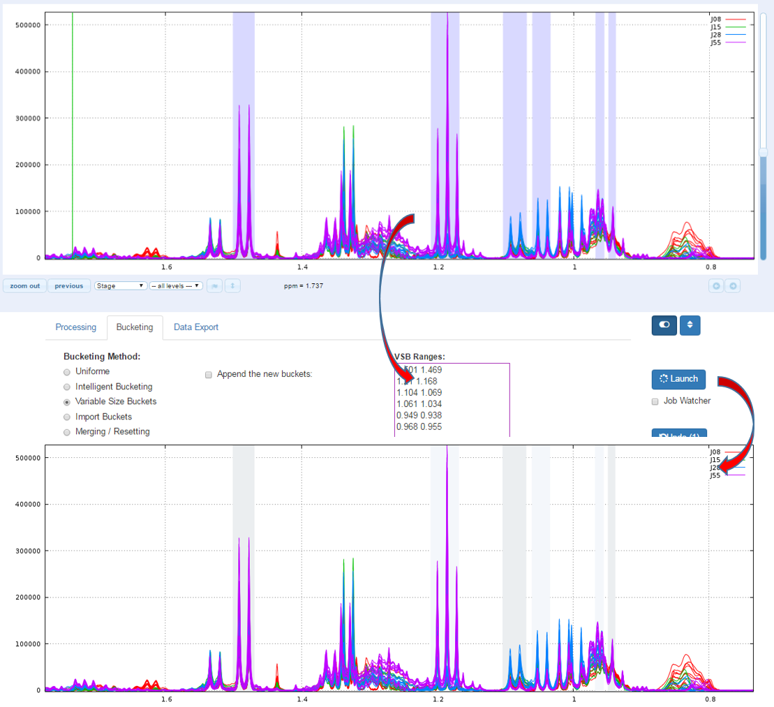

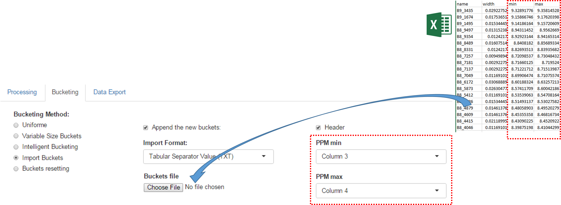
An exported buckets table can be imported into NMRProcFlow in order to retrieve the same bucketing obtained in a previous work session
How to proceed (see fig below)
- Choose the format corresponding of the imported file
- Check if the imported file have an header line or no
- Choose the corresponding columns for the lower and upper ppm bounds of the buckets.
- Check if imported buckets will be append to those already defined or not. If not, all buckets previously defined will be erased.
- Then launch

Data Export
Before exporting, in order to make all spectra comparable each other, we have to account for variations of the overall concentrations of samples. In NMR metabolomics, the total intensity normalization (called the Constant Sum Normalization) is often used so that all spectra correspond to the same overall concentration. It simply consists to normalize the total intensity of each individual spectrum to a same value. But other methods such as Probabilistic Quotient Normalization [Dieterle et al. 2006] assumes that biologically interesting concentration changes influence only parts of the NMR spectrum, while dilution effects will affect all metabolite signals. Probabilistic Quotient Normalization (PQN) starts by the calculation of a reference spectrum based on the median spectrum. Next, for each variable of interest the quotient of a given test spectrum and reference spectrum is calculated and the median of all quotients is estimated. Finally, all variables of the test spectrum are divided by the median quotient. We suggest the reference [Kohl et al. 2012] as a good review that could be read with great profit.
An internal reference can be used to normalize the data. Typically, an Electronic reference (ERETIC) can be used for that (see Akoka et al. 1999). Integral value of each bucket will be divided by the integral value of the PPM range given as reference..
How to proceed (see fig below)
- Choose a Normalization Method
- Choose an Export Format
- Choose the threshold of the Signal/Noise Ratio (SNR) so that the buckets having a lower average integration will be excluded.
- Specify if necessary, the PPM range of the internal reference signal (typically, the ERETIC signal). Otherwise, leave empty this box.
- Then, click on Export

After exporting, the data matrix is formatted so that we can subsequently perform statistical analysis using BioStatFlow web application. Thus the data file manipulations are minimized. See Metabolic Fingerprinting

Dieterle F., Ross A., Schlotterbeck G. and Senn H. (2006). Probabilistic Quotient Normalization as Robust Method to Account for Dilution of Complex Biological Mixtures. Application in 1H NMR Metabonomics. Analytical Chemistry, 78:4281-4290.
Kohl SM, Klein MS, Hochrein J, Oefner PJ, Spang R, Gronwald W. (2012) State-of-the art data normalization methods improve NMR-based metabolomic analysis, Metabolomics 146-160, DOI:10.1007/s11306-011-0350-z
Akoka S1, Barantin L, Trierweiler M. (1999) Concentration Measurement by Proton NMR Using the ERETIC Method., Anal. Chem 71(13):2554-7. doi: 10.1021/ac981422i.

The buckets table can be exported in order to be saved on your local space disk. Then it can be used as an association file along with the data matrix within BioStatFlow, or be imported into NMRProcFlow (see below)

The exported buckets table can be imported into NMRProcFlow in order to retrieve the same bucketing obtained in a previous work session. See Import Buckets

The Signal-Noise Ratio (SNR) matrix can be exported, as shown below

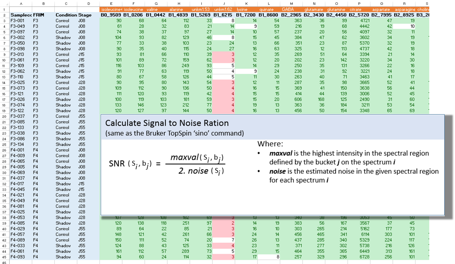
See online some slides about the SNR Exporting

After the processing and bucketing steps, NMRProcFlow allows users to export all data needed for the quantification in a same XLSX workbook. Two workbook templates were currently available: A simple one and a template dedicated for the quantification.
- The simple template just aggregates the buckets table, the SNR matrix and the data matrix, each data type being within a separate tab.
- The 'qHNMR' template, in the same way as the simple template aggregates information like the samples table, the buckets table, the SNR matrix and the data matrix within separate tabs, but also includes another tab with the pre-calculated quantifications according to a formula from data provided in the others tabs. Some information are set by default in both 'samples' and 'buckets' tabs. Just adjust them with the appropriate values and the quantifications within the eponymous tab will be automatically updated.
How to proceed (see fig below)
- Choose a template type
- Choose a Normalization Method
- Choose the threshold of the Signal/Noise Ratio (SNR) so that the buckets having a lower average integration will be excluded.
- Specify if necessary, the PPM range of the internal reference signal (typically, the ERETIC signal). Otherwise, leave empty this box.
- Then, click on Export
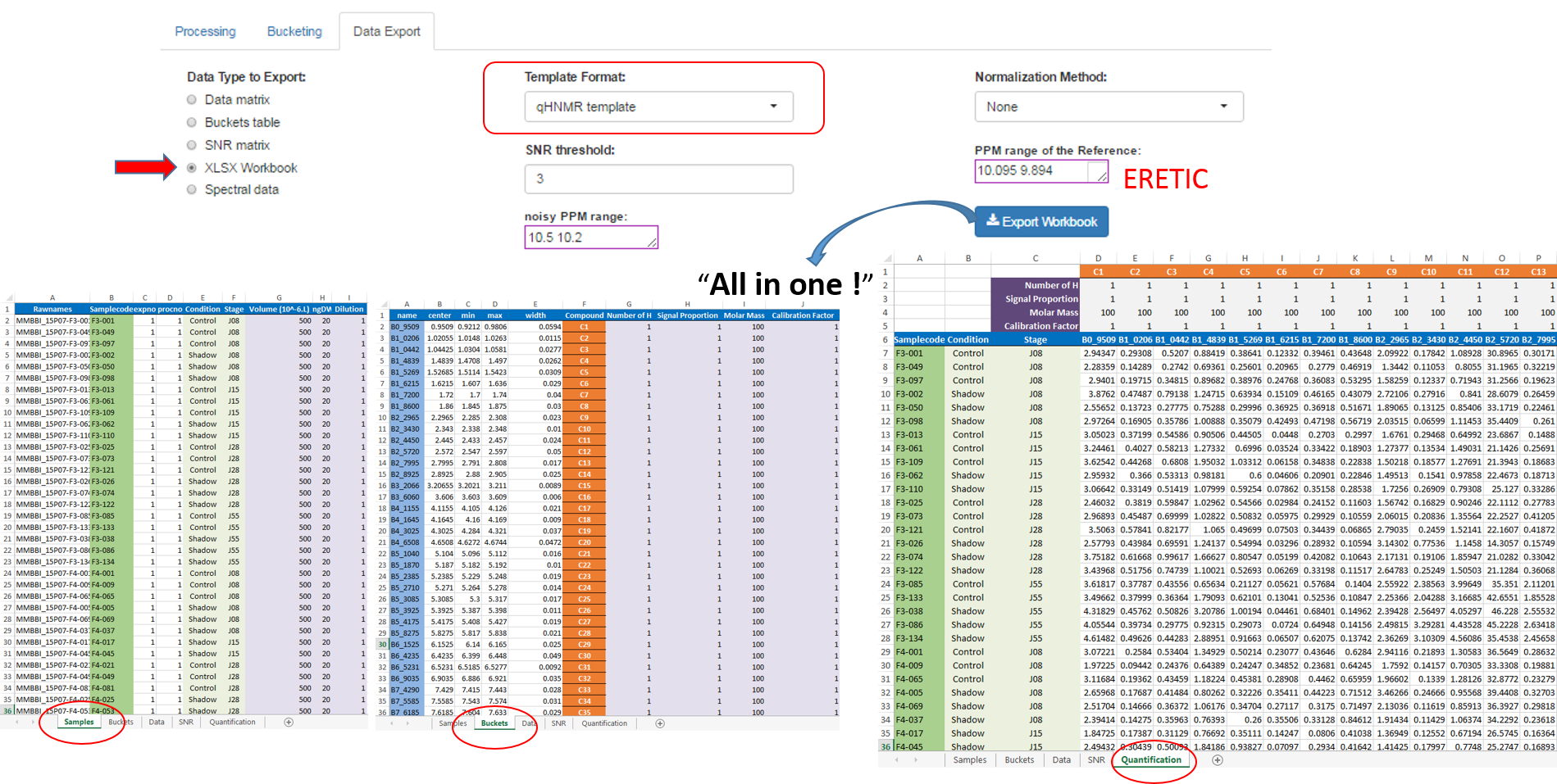
See Targeted Metabolomics for further information

Restore a session
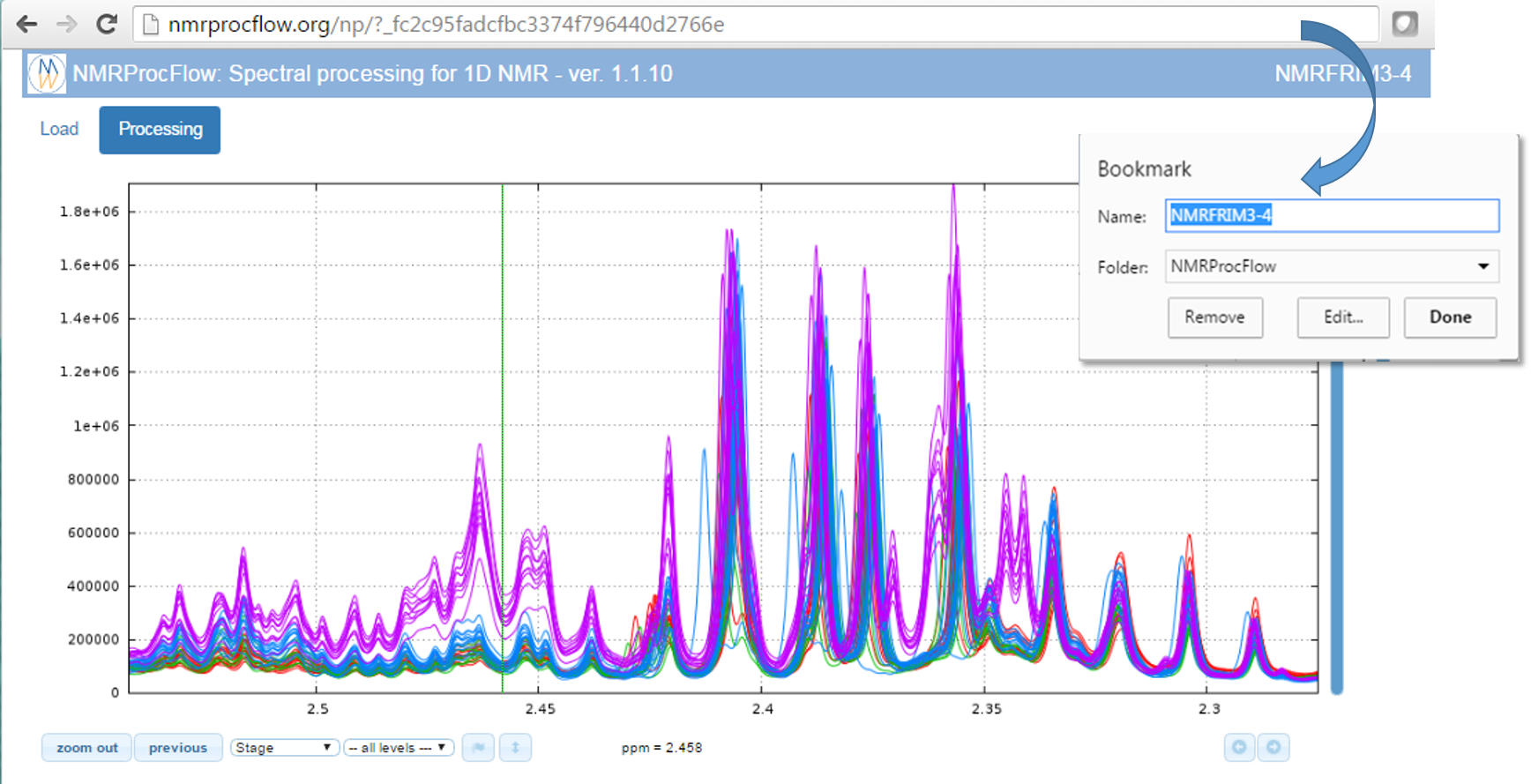
1) Bookmark the URL corresponding to your session as shown in the figure below (Chrome browser). Instead of the URL itself, the chosen name is based on the ZIP name you have upload in your session, giving an easy mnemonic way to retrieve the bookmark in your list (sometimes crowded)
2) Recovering your working session in the same state as you left after few hours or days, depending on the period of the automatic cleaning process.
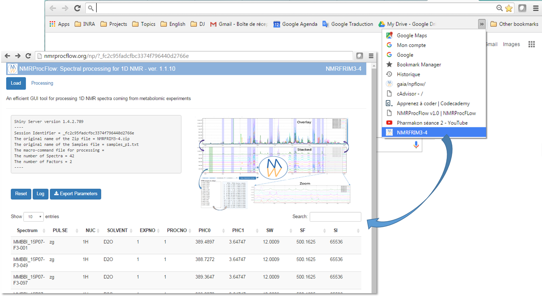

NMRProcFlow does not manage sessions in a medium or long term period.
- An automatic cleaning process has been implemented to periodically purge the working sessions with no activities over the past few days
The choice was to make a processing tool on the fly
- No need for large disk space and no need to backup
NMRProcFlow allows users to save on their own space a minimal set of small files ...

... in order to recover / replay their session
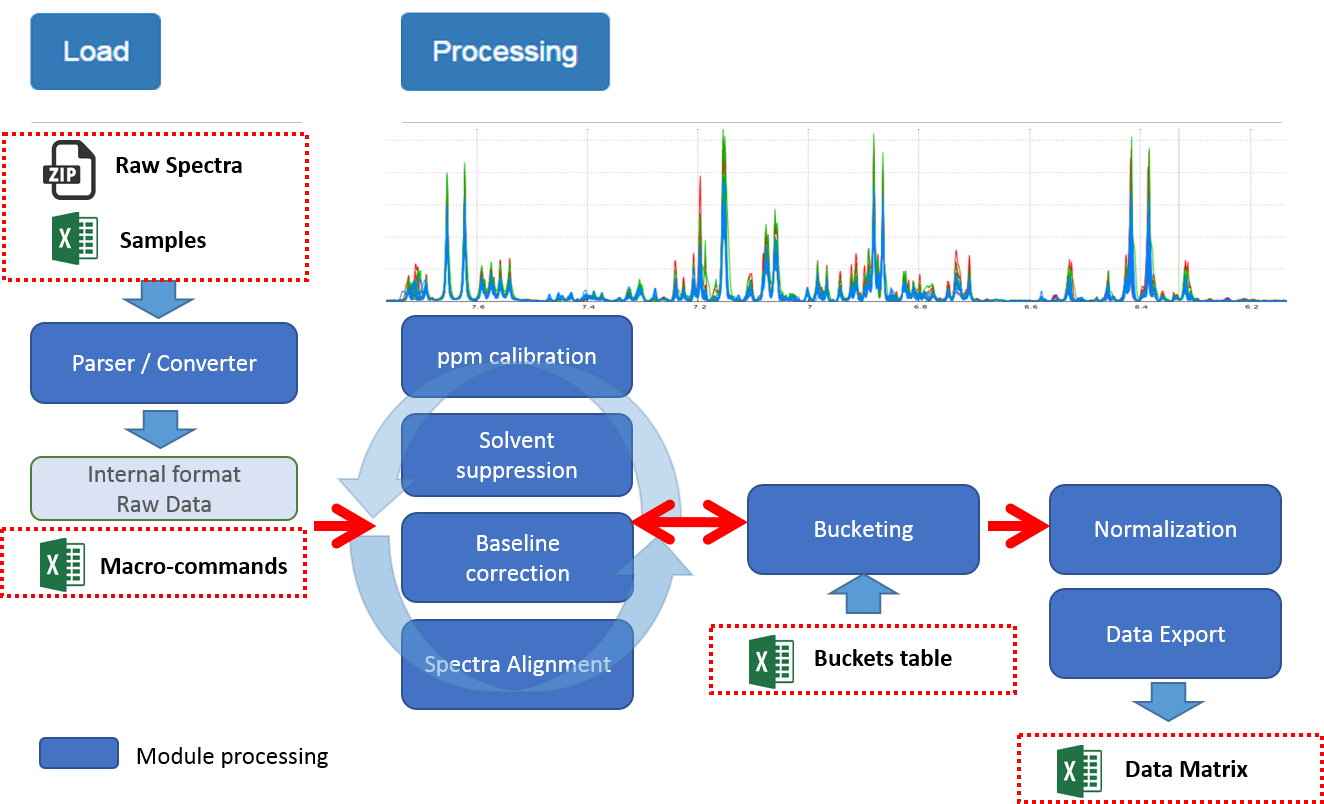
How to regenerate a session with the same treatment ?
1) Before existing your session, just export a file of macro-commands

To save the processing commands in order to replay them later on the same or similar NMR spectra, just click on the CMD button
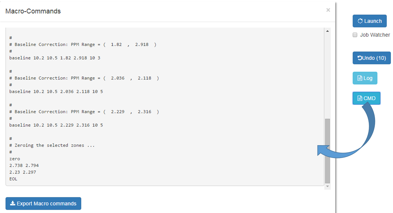
As shown in the figure below, all processing commands previously launched are logged into a macro-command file which can be saved on your local disk.
2) Replay the same processing workflow ... few months later
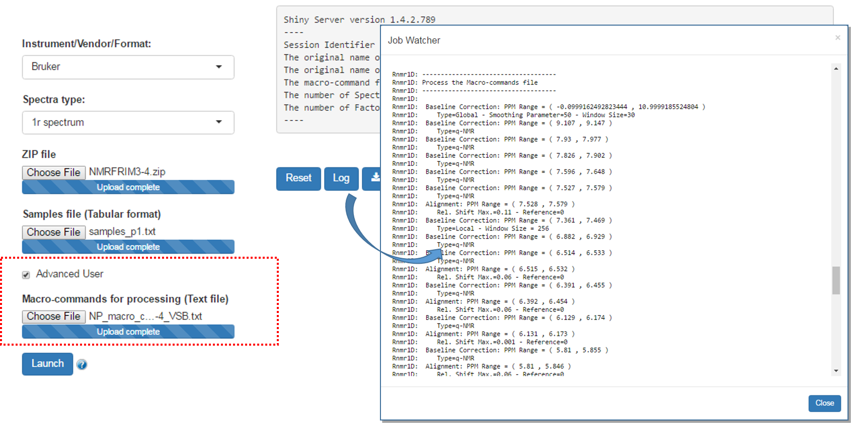
An option allows advanced users to submit a file of macro-commands along with the ZIP file of the raw spectra so that we can process the 1D NMR spectra in the same way as we proceeded them in a previous work session.

Batch mode execution
NMRProcFlow allows experts to build their own spectra processing workflows, in order to become models applicable to similar NMR spectra sets, i.e. stated as use-cases.
In the Replay the same processing workflow section, we have seen how to export a macro-commands file in order to be replayed in the NMRProcFlow GUI, i.e. in interactive mode. Now the idea as depicted in the figure below, is to consider the macro-commands file as a processing model that can be applied on other subsets and replayed in batch mode.
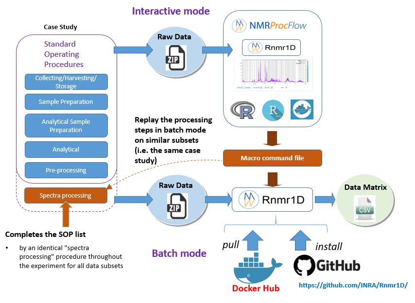
By extension, we consider the implementation of NMR spectra processing workflows executed in batch mode as relevant provided that we want to process in this way very well-mastered and very reproducible use cases, i.e. by applying the same Standard Operating Procedures (SOP).
- Interactive mode: A subset of NMR spectra is firstly processed in interactive mode using NMRProcFlow having a NMR spectra viewer to allow the expert eye to disentangle the intertwined peaks, in order to build a well-suited workflow. This mode could be also named the 'expert mode'.
- Batch mode: Then, other subsets that could be regarded as either similar or being included in the same case study, can be processed in batch mode (See below the two options)
* To run the R Rnmr1D package within a R session, go to the github repository https://github.com/INRA/Rnmr1D. You can also see the online vignette that illustates the Rnmr1D package features
Cloud-based Metabolomics Data Processing
* To run the Rnmr1D application on a Cloud Research Environment (CRE), go to the Galaxy Portal of the EU PhenoMenal H2020 project.
* See the presentation "NMRProcFlow combined with the computing power of a Cloud Research Environment".

Examples in action
Exemple 1: Spectra alignment performed on a ppm window
This example is based on 1H NMR spectra from leaves of grapevine (D2O Solvent, NOESY Pulse sequence, pH 6, NMR 500MHz)
Exemple 2: A complete processing performed on a ppm window
Here is a subset of NMR spectra (Brain of Mice, D2O Solvent, NOESY Pulse sequence, pH 4, NMR 600MHz) within a ppm range
Example coming from MetaToul Platform: Cabaton, N. et al (2013).Effects of low doses of bisphenol A on the metabolome of perinatally exposed CD-1 mice. Environmental Health Perspectives, 121 (5), 586-593. DOI : 10.1289/ehp.1205588
For more details, see W4M - NMR Mus musculus dataset
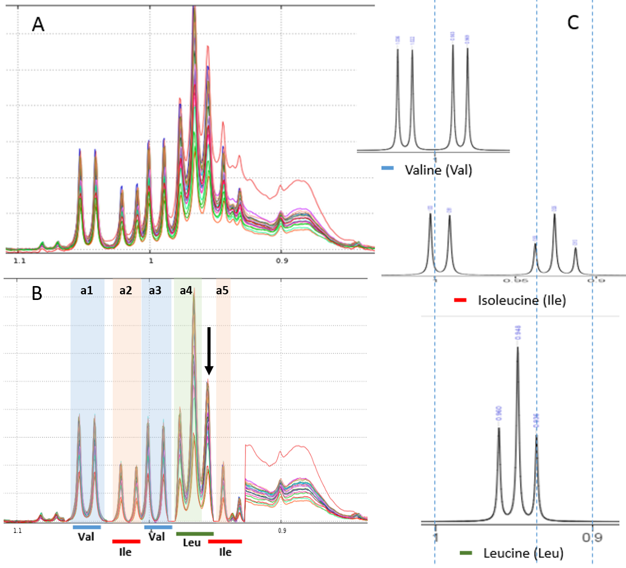
Before applying the several processing steps

After treatments

Among the performed treatments:
- there was an overall correction of the base line, then several local corrections to eliminate the effect of the presence of proteins within the analytical samples;
- thereafter, a realignment was carried out on the two areas between 6.98 and 7.08 ppm;
- finally a bucketing called "intelligent binning" was performed
Exemple 3: Another complete processing performed on a ppm window
Here is a subset of NMR spectra (48 1H-NMR spectra of Tomato pericarp extracts, D2O Solvent, single Pulse sequence, pH 6, NMR 500MHz) within a ppm range. To download the complete dataset, see "A full data set as example".
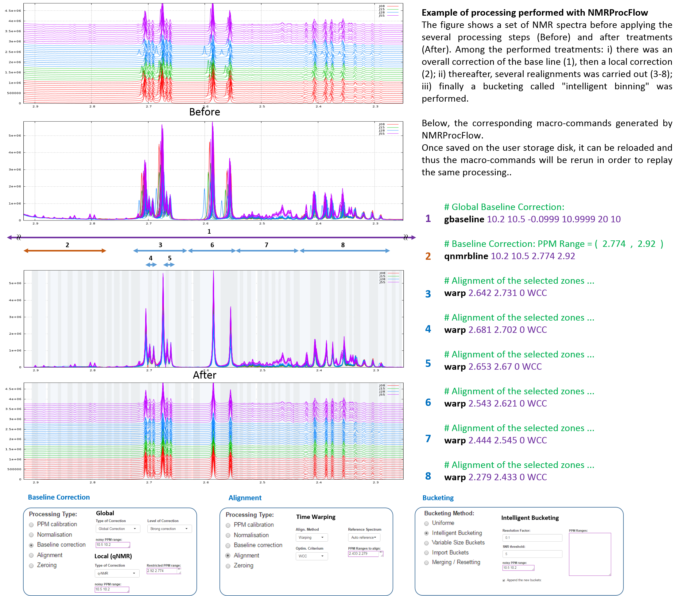

Example of full 1H-NMR data set
To assess the influence of the environment on fruit metabolism, tomato (Solanum lycopersicum 'Moneymaker') plants were grown under contrasting conditions (optimal for commercial, shaded production) and locations. Samples were harvested at nine stages of development, and 36 enzyme activities of central metabolism were measured as well as protein, starch, and major metabolites, such as hexoses, sucrose, organic acids, and amino acids.
For more details, see FRIM - Fruit Integrative Modelling, an ERASysBio+ projet, and the references given below.
The available dataset for download can be simply depicted and summarized by the following figure:

References
Bénard C., Bernillon S., Biais B., Osorio S., Maucourt M., Ballias P., Deborde C., Colombié S., Cabasson C., Jacob D., Vercambre G., Gautier H., Rolin D., Génard M., Fernie A., Gibon Y., Moing A. 2015 Metabolomic profiling in tomato reveals diel compositional changes in fruit affected by source-sink relationships. Journal of Experimental Botany Vol. 66, No. 11 pp. 3391–3404 doi:10.1093/jxb/erv151
Beauvoit B., Colombié S., Monier A., Andrieu M.-H., Biais B., Bénard C., Chéniclet C., Dieuaide-Noubhani M., Nazaret C., Mazat J.-P., Gibon Y. (2014). Model-assisted analysis of sugar metabolism throughout tomato fruit development reveals enzyme and carrier properties in relation to vacuole expansion. Plant Cell 26: 3224–3242
Biais B, Bénard C, Beauvoit B, Colombié S, Prodhomme D, Ménard G, Bernillon S, Gehl B, Gautier H, Ballias P, Mazat J-P, Sweetlove L, Génard M, Gibon Y. 2014. Remarkable reproducibility of enzyme activity profiles in tomato fruits grown under contrasting environments provides a roadmap for studies of fruit metabolism. Plant Physiology 164, 1204-1221.
Colombié S, Nazaret, Bénard C, Biais B, Mengin V, Solé M, Fouillen L, Dieuaide- Noubhani M, Mazat J, Beauvoit B, Gibon Y. 2015. Modelling central metabolic fluxes by constraint-based optimization reveals metabolic reprogramming of developing tomato fruit. The Plant Journal 81, 24-39.

For 1H-NMR profiling, polar metabolites, were extracted from the ground lyophilised samples as previously described (Biais et al., 2009; Moing et al., 2004) with minor modifications. Frozen powdered samples were lyophilised and polar metabolites were extracted from 20 mg of lyophilised powder with an ethanol-water series at 80°C. The supernatants were combined, dried under vacuum and lyophilised. Two technical replicates were prepared for each fruit sample. Each lyophilised extract was solubilised in 500 µL of 250 mM potassium phosphate buffer solution at apparent pH 6.0, 5 mM ethylene diamine tetraacetic acid disodium salt (EDTA), in D2O, titrated with KOD solution to pH 6.00 ±0.02 when necessary, and lyophilised again. The lyophilised titrated extracts were stored in darkness under vacuum at room temperature, before 1H-NMR analysis was completed within one week.
Before 1H-NMR analysis, 500 µL of D2O with sodium trimethylsilyl [2,2,3,3-d4] propionate (TSP, 0.01% final concentration for chemical shift calibration) were added to the lyophilised titrated extracts. The mixture was centrifuged at 10,000 g for 5 min at room temperature. The supernatant was then transferred 1 into a 5 mm NMR tube for acquisition. Quantitative 1H-NMR spectra were recorded at 500.162 MHz and 300 K on a Bruker Avance III spectrometer (Wissembourg, France) using a 5-mm broadband inverse probe, a 90° pulse angle and an electronic reference for quantification (Biais et al., 2009; Mounet et al., 2007).
The assignments of metabolites in the NMR spectra were made by comparing the proton chemical shifts with literature (Fan, 1996; Mounet et al., 2007) or database values (MeRy-B, HMDB), by comparison with spectra of authentic compounds recorded in the same solvent conditions (in-house library) and by spiking the samples. 1H-1H COSY NMR experiments were acquired for selected samples for assignment verification.
For absolute quantification of metabolites, four calibration curves (glucose and fructose: 1.25 to 50 mM, glutamate and glutamine: 0 to 15 mM) were prepared and analysed under the same conditions. The glucose calibration was used for the absolute quantification of all compounds, as a function of the number of protons of selected resonances except fructose, glutamate and glutamine quantified using their respective calibration curve.
References
Biais B, Allwood JW, Deborde C, Xu Y, Maucourt M, Beauvoit B, Dunn WB, Jacob D, Goodacre R, Rolin D, Moing A. 2009. H-1 NMR, GC-EI-TOFMS, and Data Set Correlation for Fruit Metabolomics: Application to Spatial Metabolite Analysis in Melon. Analytical Chemistry 81, 2884-2894.
Fan TWM. 1996. Metabolite profiling by one- and two-dimensional NMR analysis of complex mixtures. Progress in Nuclear Magnetic Resonance Spectroscopy 28, 161- 219.
Moing A, Maucourt M, Renaud C, Gaudillere M, Brouquisse R, Lebouteiller B, Gousset-Dupont A, Vidal J, Granot D, Denoyes-Rothan B, Lerceteau-Kohler E, Rolin D. 2004. Quantitative metabolic profiling by 1-dimensional H-1-NMR analyses: application to plant genetics and functional genomics. Functional Plant Biology 31, 889-902.
Mounet F, Lemaire-Chamley M, Maucourt M, Cabasson C, Giraudel JL, Deborde C, Lessire R, Gallusci P, Bertrand A, Gaudillere M, Rothan C, Rolin D, Moing A. 2007. Quantitative metabolic profiles of tomato flesh and seeds during fruit development: complementary analysis with ANN and PCA. Metabolomics 3, 273-288.

Input files
| File Name | Format | Description |
|---|---|---|
| NMRFRIM3-4.zip | Zipped | ZIP of the complete Bruker directory of the samples |
| samples_p1.txt | Tabular Text | the spectra list file relative to the samples |
| buckets_FRIM3-4.txt | Tabular Text | the buckets table file |
| NP_macro_cmd_NMRFRIM3-4.txt | Raw Text | the macro-command file |
Calibration files
| File Name | Format | Description |
|---|---|---|
| FruGlu.zip | Zipped | ZIP of the complete Bruker directory of the Fructose-Glutamate calibration-curve |
| FruGlu_pdata2.txt | Tabular Text | the spectra list file relative to the Fructose-Glutamate calibration-curve |
| buckets_FruGlu.txt | Tabular Text | the buckets table file the Fructose-Glutamate calibration-curve |
| GlucGln.zip | Zipped | ZIP of the complete Bruker directory of the Glucose-Glutamine calibration-curve |
| GlucGln_pdata2.txt | Tabular Text | the spectra list file relative to the Glucose-Glutamine calibration-curve |
| buckets_GlucGln.txt | Tabular Text | the buckets table file the Glucose-Glutamine calibration-curve |
| Calibration-curves.xlsx | XLSX | the XLSX workbook file of the calibration-curves |
Output files
| File Name | Format | Description |
|---|---|---|
| wb_NMRFRIM3-4.xlsx | XLSX | the XLSX workbook file of quantifications |

Step 1: Load the dataset
- Download files in the 'input files' list, namely: 'NMRFRIM3-4.zip', 'samples_p1.txt' and 'NP_macro_cmd_NMRFRIM3-4.txt'
- Start NMRProcFlow from your web browser.
- Choose 'Bruker' as Instrument/Vendor/Format, and '1r spectrum' as Spectra type.
- Then load the ZIP file and the sample file as described in the 'Data preparation phase' section
- Before launchning, you have also to load the macro-command file in the form for advanced user as described in the 'Replay the same processing workflow' section
- Finaly, click on the 'Launch' button'
Step 2: Import the bucket table
- Download the bucket table file 'buckets_FRIM3-4.txt'.
- Import the bucket table as described in the 'Bucketing' section. Don't forget to select the 'Tabular Separator Value' as the import format.
Step 3: Export the XLSX workbook for quantification
- Download the XLSX workbook file 'wb_NMRFRIM3-4.xlsx'.
- Export the XLSX workbook for quantification as described in the 'Data Export' section

Download
There are three ways to install NMRProcFlow, depending on the type of installation.

|
 |
If you want to install NMRProcFlow on your desktop PC , laptop or netbook, then the best solution is to use a virtualization platform like Oracle VirtualBox |

|
 |
If the installation is to be done on a Linux server (for instance within an already created Virtual Machine with Docker properly installed), then undoubtedly, the best solution is to use Docker containers. |

|
 |
If you don't wish to install NMRProcFlow locally, you could install it on a Cloud |

Virtual Appliance
We provided virtual appliance so that users can install and use NMRProcFlow on their own computer, enabling them to process sensitive and confidential data, and also with a larger data size (the size of the ZIP is limited to 200 MB on the online version).
-
VirtualBox
Download the corresponding zipped virtual disk (VDI) - npflow_vbox_vdi_x64.7z (7zip format - LZMA2:24 Method - Compress rate: 26% - 898 Mo).
You can download the Oracle VM VirtualBox software Here along with the Oracle VM VirtualBox Extension Pack
Tested and valided with Oracle VM VirtualBox 5.1.10 under Windows 7 Pro and Windows 10 Pro
-
Warning: Enable hardware virtualization features
Modern CPUs include hardware virtualization features that help accelerate virtual machines created in VirtualBox, VMware, Hyper-V, and other apps. But those features aren’t always enabled by default. You need to ensure that this feature is enabled on your PC / Laptop. If not, you have to enable it. Many online helps exist, and we have selected the following:
How to Enable Intel VT-x in Your Computer’s BIOS or UEFI Firmware
-
Note for Windows 10 Pro
Disable the Hyper-V feature otherwise the virtual machine platforms do not work in 64-bit mode (See Here)
Use only VirtualBox from version 5.1.10 or higher
-
Note for Mac OS X 10.x
We have proceed ourselves no installation tests on Mac OS X 10.x but severals users have successful installed NMRProcFlow using VirtualBox 5.1.10 or higher. Many online helps exist, and we have selected the following:
Download 7zX for Mac OS otherwise The Unarchiver works well.

Docker Images
Warning: requires a little bit IT skills
What is Docker?
Docker is a tool designed to make it easier to create, deploy, and run applications by using containers. Containers allow a developer to package up an application with all of the parts it needs, such as libraries and other dependencies, and ship it all out as one package. By doing so, thanks to the container, the developer can rest assured that the application will run on any other Linux machine regardless of any customized settings that machine might have that could differ from the machine used for writing and testing the code. For more details, see opensource.com/resources/what-docker
Installation
Requirements: a recent OS that support Docker (see How to install Docker or Create a VM with Docker-Machine).
- About Docker on Ubuntu 16.04, See how-to-install-and-use-docker-on-ubuntu-16-04
- About Docker on CentOS 7, See how-to-install-and-use-docker-on-centos-7
- About Docker on MacOS 10.11 or newer, See Docker Community Edition for Mac, then Install and run Docker for Mac
Get the docker image
- Pull the docker image from DockerHub (may take a while depending on your network speed and the traffic)
$ sudo docker pull nmrprocflow/nmrprocflow
Create minimal configuration file:
- npflow.conf
# The URL root of the PROXY if applicable
PROXY_URL_ROOT=

# Duration (in days) of validity of a session
# before its destruction (counted from the last change)
PURGESESSIONS=2

# Max ZIP size (Mo)
MAXZIPSIZE=400

# NB CORES (0 means Auto)
CORES=0

# User connexion management
# 0 : no connexion management
# 1 : connexion management based on the /opt/data/conf/userlist file
#     Its structure is one user per line and each line following the format:
#        login;LastName;FirstName;Country;Institution;Email;Password
#     a minimal set of this 'userlist' file could be: npflow;;;;;;nppass
USRCONMGR=0
Create a shell script file (Linux):
#!/bin/bash
MYDIR=`dirname $0` && [ ! `echo "$0" | grep '^\/'` ] && MYDIR=`pwd`/$MYDIR

DATADIR=/opt/data

# nmrspec Container
PORT=8080
IMAGE=nmrprocflow/nmrprocflow
CONTAINER=npflow
CONF=$MYDIR/npflow.conf

CMD=$1

# If you use a local directory, first you have to create the $DATADIR directory
VOLS="-v $DATADIR:/opt/data"

usage() { echo "usage: sh $0 start|stop|ps|restart|logs|update";  exit 1; }

case "$CMD" in
   start)
        # run NMRProcFlow
        sudo docker run -d --env-file $CONF $VOLS -p $PORT:80 --name $CONTAINER $IMAGE

        # show Logs
        sudo docker logs $CONTAINER
        ;;
   stop)
        LIST=$(sudo docker ps -a | grep $IMAGE | cut -d' ' -f1)
        sudo  docker stop $LIST
        sudo  docker rm $LIST
        ;;
   restart)
        ( sh $0 stop; sh $0 start)
        ;;
   logs)
        sudo docker logs $CONTAINER
        ;;
   ps)
        sudo docker ps | head -1
        sudo docker ps | grep $IMAGE
        ;;
   update)
        sudo docker pull $IMAGE
        ;;
   *) usage
      exit 2
esac
Start the application (Linux)
sh ./npflow.sh startThen, in your favorite web browser, check on (You have to enable JavaScript functionalities within your web browser):
http://<your_vm_host>:8080/npflow/Stop the application (Linux)
sh ./npflow.sh stopStatus of the application (Linux)
sh ./npflow.sh psView logs of the application (Linux)
sh ./npflow.sh logsNGINX configuration (Linux)
For avanced users: In case you would like to use a proxy server, the better is to install and set NGINX, an HTTP and reverse proxy server.
In the /etc/nginx/conf.d/my-site.conf, you should add three 'location' sections as shown below:
server {
    listen 80 default;
    server_name $host;

    ...

    location /nv/ {
        proxy_pass http://localhost:8080/nv/;
    }

    location /npwatch/ {
        proxy_pass http://localhost:8080/npwatch/;
    }

    location /np/ {
        proxy_pass http://localhost:8080/npflow/;
        proxy_redirect http://localhost:8080/npflow/ $scheme://$host/npflow/;
        proxy_http_version 1.1;
        proxy_set_header Upgrade $http_upgrade;
        proxy_set_header Connection "upgrade";
        proxy_set_header Host $host;
    }

    ...

}
Firewall/Antivirus Issues
NMRProcFlow uses R Shiny for its Graphical Unit Interface (GUI). This latter relies on SockJS based on the HTTP WebSocket protocol to facilitate communication between the browser and the server. Unfortunateley, unencrypted WebSocket traffic is often filtered or blocked. First, you can test if WebSockets work for you.
So, if you get a shaded screen, it's probably due to either your antivirus, your firewall or if you work within a VPN. To solve this problem, add the URL http://nmrprocflow.org/np/ as an exception (ie an exclusion for the application of the security rules), or as a trusted site, according to your software tools available on your workstation.
The antiviruses known to enforce strict rules for the WebSocket protocol are for example: Kaspersky, Avast
Do not hesitate to ask to your IT administrator for explaination how to proceed.

Changelog
Thanks to the users who send us the encountered issues and bugs, NMProcFlow can thus be made more reliable. When an update is performed, it includes the online version, Docker containers as well as the Virtual Machine.
Version 1.4.48 - April 10, 2026
* Check if the spectra are of different sizes. If not, you can download the list of spectra and their corresponding information.Macro command saving for bucketing (unif, aibin, erva & vsb). Import, merge, and reset operations are not saved.Version 1.4.42 - October 31, 2025
   * Macro command saving for bucketing (unif, aibin, erva & vsb). Import, merge, and reset operations are not saved.
   * Addition of the possibility to simply apply a ppm shift to recalibrate the spectra.
Version 1.4.30 - July 28, 2025
   * Phasing improved for CPMG and NOESY sequences
   * Support for CP sequences (used for solid state NMR)
   * Acceleration of the spectra matrix generation step during pre-processing
Version 1.4.26 - April 8, 2025
   * Addition of bucketing by the ERVA method (Jacob et al. 2013,Analytical and Bioanalytical Chemistry - doi: 10.1007/s00216-013-6852-y)
   * Improvement of zero-order phasing in the presence of a calibration signal (TSP, TMSP, DSS)
   * Allows you to change the order of baseline correction (local method). Previously, we only had order one by default.
   * Visualization of distance in Hz when selecting an interval on spectra
   * Support for Magritek SpinSolve spectra (still experimental due to lack of data)
* Fixes several minor bugs...Version 1.3.08 - September 3, 2019
* Fixed an issue when exporting data matrix especially when the samples file is provided.Macro-command files compatibility between versions 1.2.x and 1.3.x
   * In the case where first-order phasing is necessary, you may need to add in the first line of the macro-command file the criterion:
   * either CRIT1=1; for "Absolute positives" or CRIT1=0; for "Negative values" (Use for that a simple text editor)
   * To know which one is better, test with your spectrum set without the macro-command file.
Version 1.3.02 - August 2, 2019
   * NMR spectra of phosphorus (31P) is now supported
   * Now displays the full ppm range of spectra. This makes it possible to support the NMR spectra of phosphorus (31P).
   * Allows bucketing in ppm areas with negative values. (required for phosphorus).
   * Phase correction improvement
Version 1.2.30 - May 10, 2019
   * Adds the possibility to make a first reset without having to reload the ZIP file and also to login again.
     This makes it easier to test several preprocessing settings.
Version 1.2.28 - March 5, 2018
* RS2D SPINIt format is now supported for both FID and 1r spectrumVersion 1.2.26 - October 29, 2018
   * During the preprocessing phase, in case of failure on one or more spectra, these latter are not
     taken into account in order to avoid stopping at an error so that the process can continue with all
     the remaining spectra.
   * The visualization of the spectra has been made even more fluid by drastically improving its speed.
     This also results in a very slight loss of quality of the images produced. But it is possible to
     restore the previous quality (a button allows you to switch between SD - Small Definition and
     HD - High Definition). Thus sets of more than 300 spectra can be visualized with fluidity.
   * Added an animated logo during exports (which can take several seconds sometimes) serves to indicate
     that the current running process.
Version 1.2.24 - June 28, 2018
   * In order to calibrate the ppm scale when a set of spectra has not been acquired with the same locking
     frequency, we have added a parameter in the preprocessing panel that allows to ignore the spectral region
     center parameter due to the fact it exhibes large differences between spectra ('O1' for Bruker,'tof' for
     Varian and'x_offset for Jeol). Instead, we choose an arbitrary zero at the third of the sweep width
    (i.e. SW in Hertz).
Version 1.2.22 - May 24, 2018
   * To efficiently align some tricky ppm zones, the possibility to shift these zones on one or several spectra
    (corresponding to the same factor level) has been added.
   * More robust mouse management (movements and events)
     Now it is possible to move the mouse forward / backward to select ppm zones.
     Prevents the cursor loss
   * Fix some other minor bugs
Version 1.2.18 - March 1, 2018
   * Jeol JDF format is now supported
   * Improvement of the Zero order phasing (needless in most time to proceed the First order phasing).
   * Improvement of the ppm scale calibration (usefull when no calibration with TSP/DSS)
   * Ease the preprocessing with differents parameters without need to upload again the ZIP file.
Version 1.2.12 - Oct 18, 2017
* Fixed bug when exporting the data matrix export (some bucket columns may be disappeared)Version 1.2.10 - August 7, 2017
   * Fixed bug when exporting the quantification workbook (column offsets could occured depending on the SNR value)
   * Implementation of the complete normalisation during the processing step (i.e. applied on the spectra based on selected ppm ranges).
Version 1.2.8 - June 15, 2017
   * Fixed bug with FIDs coming from Bruker having a number of points not equal to a power of 2
   * Fixed bug with FIDs coming from Agilent/Varian having intensities coded as float32
   * Improved the algorithm for phase correction
Version 1.2.6 - March 27, 2017
* Fixed the bug when exporting the 'q-HNMR' WorkBook This occurred in the absence of factors.Version 1.2.5 - Feb 15, 2017
* Improved the algorithm for phase correction (rewritten in C++)Version 1.2.2 - Jan 20, 2017
  * Added a spectra pre-processing module in order to support the FID (Free Induction Decay) directly as input.
    Two major vendors are supported, namely Bruker GmbH & Agilent Technologies (Varian), as well as the new nmrML format.
  * Added the airPLS baseline correction  (implementation based on sparse matrices)
  * Added the "CluPA" alignment method (R package 'speaq'), slightly adapted to be more efficient
  * Added an alternative way to manage the capture mode using the "Ctrl Key"
Version 1.1.22 - Dec 10, 2016
   * Added the "Time Warping" alignment method (R package 'ptw')
   * Added the data exportation within XLSX Workbooks, in particular for quantification (q-HNMR template)
   * Added the "Batch mode execution": similar subsets can be processed in batch mode
    (executed using the "rnmr1d" docker image, got from DockerHub)
Version 1.1.10 - July 11, 2016
   * The first "official" release, available online:
      -  as a web application
      -  downloadable as a Virtual Machine (VMware & VirtualBox)
      -  downloadable as a Docker image (DockerHub)

