Spectra processing

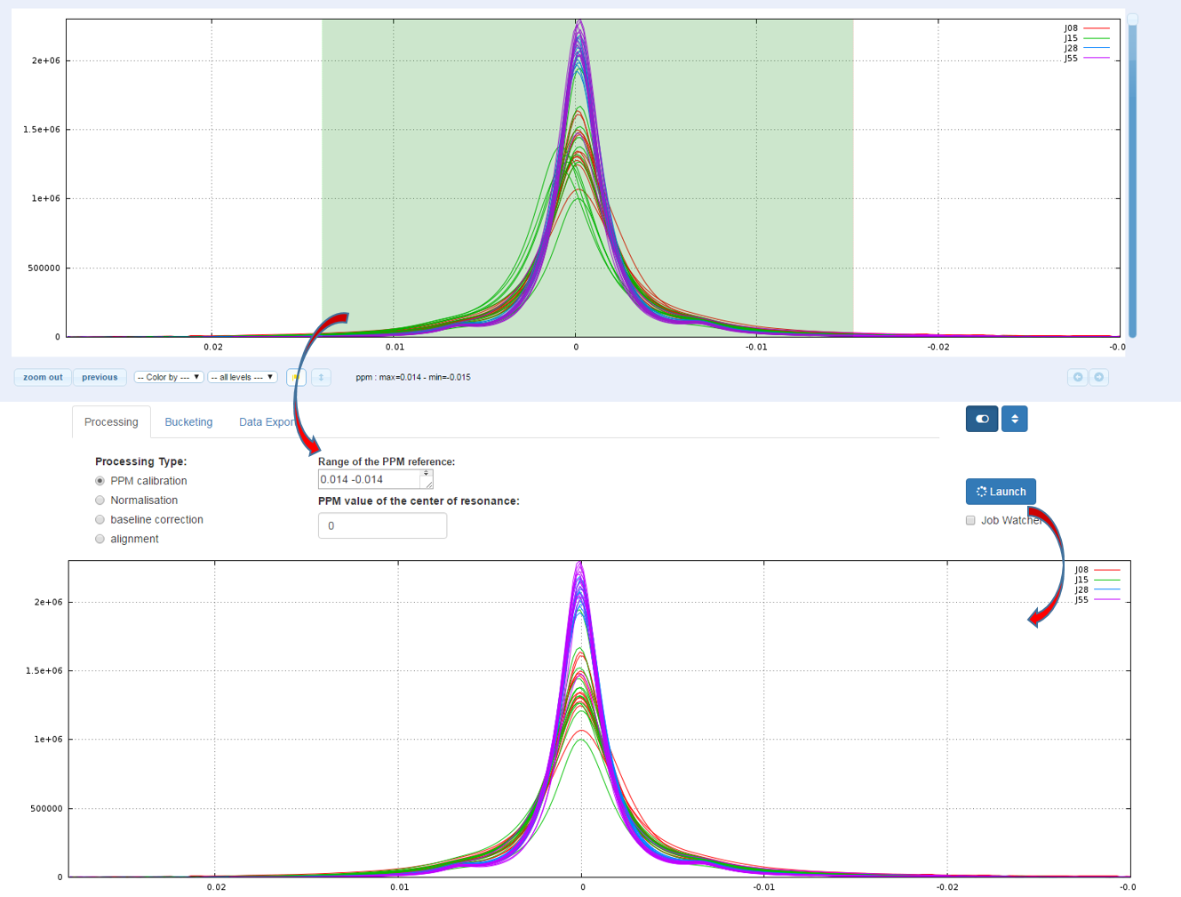
The calibration of the scale of PPM is to adjust the chemical shifts according to a known reference. The reference compound used for chemical shift (δ=0.00) is usually the sodium salt of 3-trimethylsilylpropionic acid-d4 (TSP-d4) with deuterated methylene groups. Other references standards are 2,2- 23 dimethyl-2-silapentane-5-sulfonate sodium salt (DSS) or for organic solvent trimethylsilane (TMS). But it may be any other compound such as creatinine (4.06ppm), α-glucose (5.23ppm), alanine (a doublet along with a peak at 1.488ppm), etc...

How to proceed (see fig below)

• Capture the reference peak into the ‘Range of the PPM reference’ box
• Specify the ppm value corresponding to the highest intensity of the reference peak
• Then launch

Because on the one hand the peak integration is very sensitive to baseline distortions and on the other hand the baseline distortions may not affect in the same way each spectrum, we have to apply a baseline correction.

Two types of Baseline correction were implemented: Global and Local. (For more details, see Processing methods). To be more efficient, both methods need to estimate the noise level, and by default the ppm range included between 10.2 and 10.5 ppm is taken. But you can choose another one if some signal is present in this area.

1 - Global

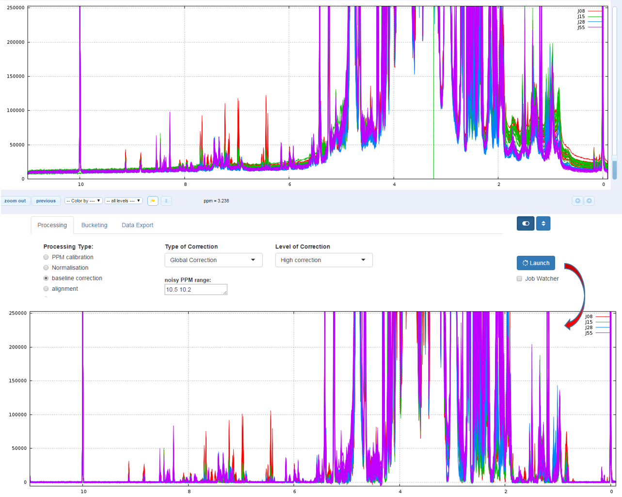
The global baseline correction was based on [Bao et al, 2012], but only two phases were implemented: i) Continuous Wavelet Transform (CWT) and ii) the sliding window algorithm. The user must choose the correction level, from 'soft' up to 'high'.

How to proceed (see fig below)

• Choose the correction level, from 'Soft correction' up to 'High correction'
• Capture the ppm range in order to estimate the noise level
• Then launch

Bao et al (2012) A new baseline correction method based on iterative method, Journal of Magnetic Resonance 218 (2012) 35-43

2 - Local

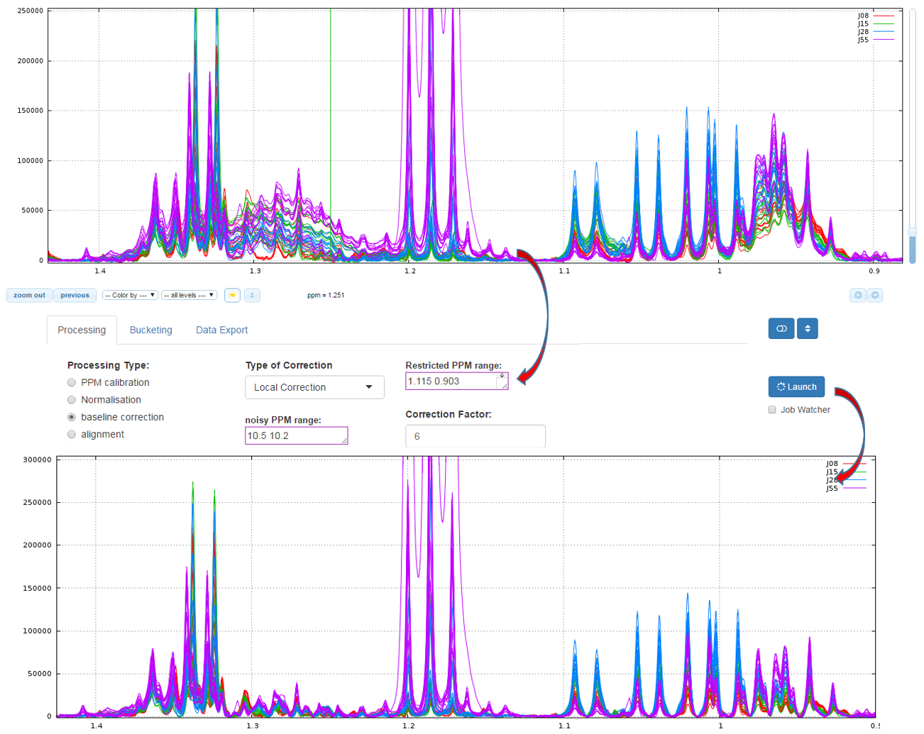
The airPLS (adaptive iteratively reweighted penalized least squares) algorithm based on [Zhang et al, 2010] is a baseline correction algorithm which works completely on its own, and that does only require a detail parameter for the algorithm, called Lambda. Because this Lambda parameter can vary within a very large range (from 10 up to 1.e+06), we converted this parameter within a more convenient scale for the user, called 'level correction factor' chosen by the user from '1' (soft) up to '6' (high). The lower this level correction factor is set the smoother baseline will be. Conversely, the higher this level correction factor is set, the more baseline will be corrected in details. To be more efficient, the algorithm needs to estimate the noise level, and it takes by default the ppm range included between 10.2 and 10.5 ppm. But you can choose another one if some signal is present in this area

How to proceed (see fig below)

• Capture the ‘Range of the PPM’ to be corrected
• Choose the correction level, from '1' up to '7'
• Capture the ppm range in order to estimate the noise level
• Then launch

Zhang Z, Chen S, and Liang Y-Z (2010) Baseline correction using adaptive iteratively reweighted penalized least squares, Analyst, 2010,135, 1138-1146. doi:10.1039/B922045C

The alignment step is undoubtedly one of the most tedious to solve. The misalignments are the results of changes in chemical shifts of NMR peaks largely due to differences in pH and other physicochemical interactions. To solve this prickly problem, we implement two alignment methods, one based on a Least- Squares algorithm and the other based on a Parametric Time Warping (PTW). Compliant with the NMRProcFlow philosophy and due to the diversity of problems encountered we chose for spectra alignment, the interactive approach. It means interval by interval, each interval being chosen by the user. (For more details, see Processing methods)

1 - Least- Squares algorithm

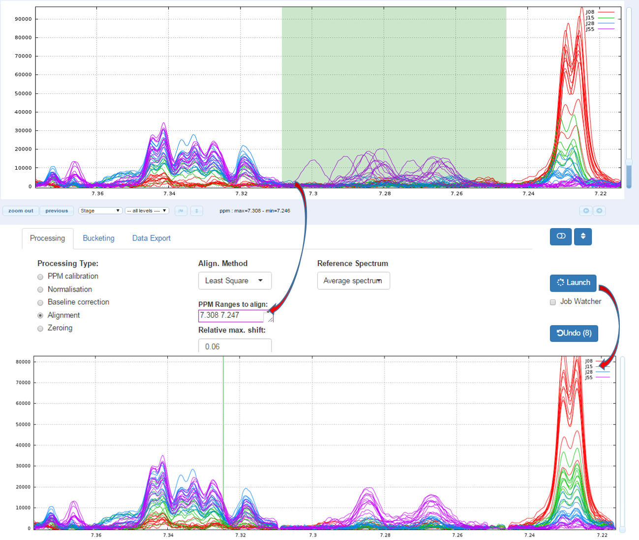
To align a set of spectra, we need to choose or to define a reference spectrum. You can align spectra either based on a particular spectrum chosen within the spectra set, or based on the average spectrum. In this latter case, the re-alignment procedure is executed three times, the average spectrum being recalculated at each time

In order to limit the relative ppm shift between the spectra to be realigned and the reference spectrum, you can set this limit by adjusting the parameter 'Relative shift max.', that sets the maximum shift between spectra and the reference. The range goes from 0 (no ppm shift allowed) up to 1 (maximum ppm shift equal to 100% of the selected ppm range)

1.1 - How to proceed (see fig below)

• Capture the ‘Range of the PPM’ to be aligned
• Set the 'Relative max/ shift'
• Choose the 'Reference Spectrum'
• Then launch

1.2 - Example showing the importance of the "Relative max. shift" parameter (see fig below)

Consider that we want to align spectra within the ppm range defined by the window as shown below:

With no way to limit the shifts between spectra, (ie. this corresponds to a relative maximum shift equal to 100%), we have the following result:

Clearly, it is not the right result. So, we set now a relative maximum shift equal to 5% (ie 0.05), and we have the right result, as shown below:

2 - Parametric Time Warping

The modus operandi for this method is very similar to the previous one, apart the "Relative max. shift" parameter that is not needed. The implementation is based on the R package 'ptw' (Bloemberg et al. 2010) and on the valuable explanations in Wehrens R. (2011).

2.1 - Example of comparison between the Least-Square and PTW methods (see fig below)

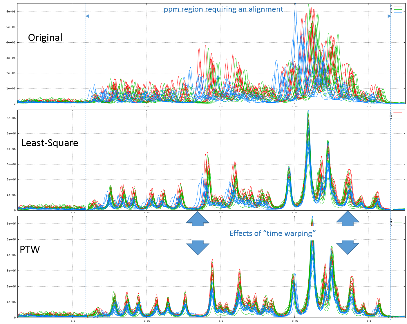
Clearly, in this example, PTW method is more efficient than a simple Least-Square approach.

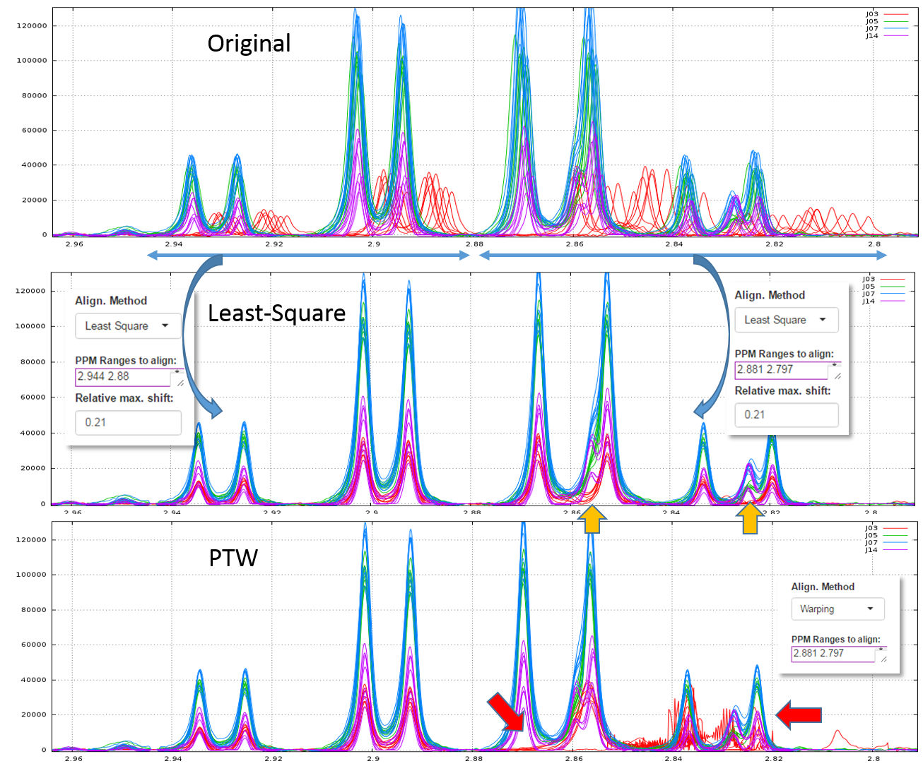
Warnings: Wehrens R. (2011) highlights the fact that (§ 3.3.2) "alignment methods that are too flexible (such as PTW) may be led astray by the presence [so by the absence] of extra peaks, especially when these are of high intensity". Therefore, a "very esthetic alignment" must not be the only quality criterion.

A good example is shown in the figure below. We first align the spectra in two steps using the Least-Square approach. The orange arrows show the absence of one peak for one stage (J03). Then, we undo the second alignment of the zone that included the problematic peak and we align again this zone using the PTW approach. All spectra are seem well-aligned apart those corresponding to the J03 stage. The red arrows show the zones where the PTW algorithm has been "astray".

T.G. Bloemberg, J. Gerretzen, H.J.P. Wouters, J. Gloerich, M. van Dael, H.J.C.T. Wessels, L.P. van den Heuvel, P.H.C. Eilers, L.M.C. Buydens, and R. Wehrens. Improved parametric time warping for proteomics. Chemom. Intell. Lab. Systems, 2010.

Wehrens R. (2011) Chemometrics with R: Multivariate Data Analysis in the Natural Sciences and Life Sciences, Ed Springer-Verlag Berlin Heidelberg